The DHS Program > Data > Calendar Tutorial
DHS Contraceptive Calendar Tutorial
Introduction
| DHS Contraceptive Calendar Tutorial PDF Updated Video 1: Completing the Contraceptive Calendar Video 2: Data Structure of the Contraceptive Calendar Programs and coding resources |
The Demographic and Health Surveys (DHS) Contraceptive Calendar Tutorial is designed to help DHS data users understand the DHS Contraceptive Calendar, its history, how it is completed in an interview, how the data are stored in the Individual Recode (IR) datasets, uses of the calendar data, and how to analyze the data.
The DHS Contraceptive Calendar Tutorial is aimed at data analysts who are very familiar with statistical software and have prior experience working with DHS datasets, and who wish to learn to analyze the DHS calendar data. This tutorial does not provide an introduction to statistical software or the DHS datasets - to learn about DHS datasets, please see the DHS Program tutorial video series.
The tutorial is split into five modules:
Module 1: What is the contraceptive (or reproductive) calendar?
Module 1 describes the DHS Contraceptive Calendar. The module provides some background and history for the DHS Contraceptive Calendar, and describes the structure of the calendar in the questionnaire and how the data are collected.
Module 2: How are the calendar data stored in datasets and how do I analyze the calendar data?
Module 2 discusses how the data are stored in the recode file, the string variables used to hold the calendar data, the coding scheme used for the calendar variables in the recode files, and how to "read" the calendar data, and introduces the three main approaches used to process the calendar data - string parsing, single month files, and event files.
Module 3: String parsing of the calendar
Module 3 describes the first approach to extracting data from the calendar, and provides four examples of the use of string parsing.
Module 4: Restructuring the calendar into a file of single months
Module 4 discusses the second approach - converting the calendar strings into a file of single months - and provides two examples of using this approach in analyzing the calendar data.
Module 5: Introduction to event files and how to use them
Module 5 introduces the third approach - creating event files - and provides an example program for producing an event file from a DHS Individual Recode (IR) file. It then provides an example of using the event file to analyze the reasons for discontinuation of contraception.
New Module 6: Contraceptive discontinuation, failure and switching rates
Module 6 tackles a subject of interest to many DHS data users - contraceptive discontinuation, failure and switching rates. It provides a description of the multiple decrement life table approach used in DHS reports, and briefly discusses single decrement life tables. It then provides an example of the contraceptive discontinuation rates using the event file.
Programs and coding resources
The tutorial comes with a set of programs written in Stata and in SPSS to support the examples.
Additionally, two videos are also available to facilitate understanding the calendar data:
- 1. DHS Contraceptive Calendar Tutorial Video Part 1: Completing the Contraceptive Calendar
- 2. DHS Contraceptive Calendar Tutorial Video Part 2: Data Structure of the Contraceptive Calendar
DHS Contraceptive Calendar Tutorial PDF
Additional information can be found in the online Guide to DHS Statistics or the PDF version. The Guide to DHS Statistics defines and explains how statistics in DHS final reports are calculated and includes several topics that use calendar data.
[Please note: Do not use the "back" button to navigate within the DHS Contraceptive Calendar Tutorial as it will take you out of the tutorial. This is because the whole tutorial loads as a single page.]Next section: 1.1 What is the calendar?
Module 1: What is the contraceptive (or reproductive) calendar?
Goal of the module: For analysts to understand what the DHS calendar is, its history, and how the data are collected.
1.1 What is the calendar?
 The DHS calendar is a month by month history of certain key events in the life of the respondent for the calendar period preceding the date of interview. It is sometimes known as the reproductive calendar or the contraceptive calendar as the main information collected in the calendar relate to reproduction and contraception. The calendar is “recent” in that only events occurring in the year of the survey plus the five1 full calendar years preceding the current year are included.
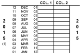
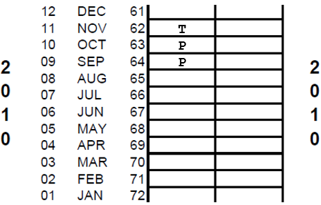
In the survey, each column of the calendar typically includes 72 boxes2 (each representing one month of time) divided into six sections (each representing one year or 12 months of time) in which to record information about the woman’s experiences with childbearing and contraceptive use. The calendar is divided into separate columns for different types of activities or event. In the current standard DHS-7 questionnaire the calendar consists of two columns:
- 1) Births, pregnancies, terminations and contraceptive use
- 2) Reasons for discontinuation of contraceptive use
The calendar collects a complete history of women’s reproduction and contraceptive use for a period of between 5 and 7 years prior to the survey. The exact length of the period covered by the contraceptive calendar varies depending on the duration of data collection, whether the survey overlapped two years and the month in which the respondent was interviewed. In most surveys the period covered by the calendar (referred to as the “calendar period”) includes the months up to the month of interview in the year of interview, plus the five1 calendar years preceding the year of interview. For example, if the interview took place in April 2015, the calendar period would cover April 2015 back to January 2010, a total of 64 months. In surveys that overlap two calendar years, where an interview is carried out in the second of those years, the period can include six calendar years prior to the year of interview. We will refer to the calendar period throughout this tutorial, meaning the period for which data were collected for a respondent. The calendar period will vary from respondent to respondent depending on the date of interview.
For each month in the calendar period a single letter or digit code is used to record information concerning the events and activities. For example, any of the following events during the calendar period would be documented:
- For each birth a letter “B” (Birth) is recorded in column 1 for the month of birth.
- For each preceding month of pregnancy a letter “P” (Pregnancy) is recorded in column 1.
- If the respondent had a miscarriage, abortion, or stillbirth, a letter “T” (Termination) is recorded in column 1 for the month the pregnancy ended, and a letter “P” (Pregnancy) is recorded for each preceding month of pregnancy.
- If the respondent used contraception in the intervening months between pregnancies, then each month of use of a contraceptive method is recorded in column 1 using the code for that method.
Below are the codes used in the DHS-7 questionnaire for column 1 (Births, pregnancies and contraceptive use) and column 2 (Reasons for discontinuation of contraceptive use):
1. Six years for surveys overlapping two years.
2. In surveys overlapping two years, an additional 12 boxes for the additional year are included in the calendar.
Next section: 1.2 How is the calendar completed in interviews?
Module 1: What is the contraceptive (or reproductive) calendar?
Goal of the module: For analysts to understand what the DHS calendar is, its history, and how the data are collected.
1.2 How is the calendar completed in interviews?
The calendar data are collected in a series of steps throughout the interview:
1) Birth history
After the birth history section has been completed in the women’s interview, the interviewer checks the number of births in the calendar period. For each birth within the calendar period the interviewer places a "B" in the first column in the row of the calendar corresponding to the month of birth and writes the child’s name to the left of the "B" code. Then the interviewer asks the respondent how many months she had been pregnant when she gave birth and records a "P" in each of the preceding months according to the duration of the pregnancy. The number of "P"s must be one less than the number of months that the pregnancy lasted as the "B" is considered to include the last month of pregnancy. This step is repeated for each birth within the calendar period. If there are twins, the birth is recorded only once in the calendar but the names of both children are recorded to the left of the month of birth.
Example: The respondent gave birth to one child in the calendar period, in November 2014. The interviewer would record a "B" in the calendar in row corresponding to November 2014. The interviewer would then ask the number of months the pregnancy lasted. If the respondent reports that she was nine months pregnant when she gave birth, the interviewer would record "P"s in each of the preceding 8 months, i.e., in the months February through October 2014, for a total of 9 months (a "B" and eight "P"s).
2) Current pregnancy
 If the interviewer ascertains that the respondent is currently pregnant and has asked the duration of pregnancy, after recording the information in the body of the questionnaire, the interviewer also records the pregnancy in the calendar. The interviewer records a "P" in column 1 of the calendar in the month of interview and in each preceding month for the duration of the pregnancy. The duration of pregnancy is recorded in completed months, so if a respondent was in her fifth month of pregnancy, this would be four completed months and four "P"s would be recorded in the calendar.
3) Terminated pregnancies
 The interviewer records any terminated pregnancies (includes miscarriages, stillbirths, and abortions) in the calendar period. For each pregnancy termination the interviewer records a ‘T’ for the pregnancy termination and a "P" for each preceding month of the pregnancy for the duration of the pregnancy. As for births, the number of "P"s is one less than the duration of the pregnancy.
Example: A respondent had a miscarriage in November 2011 and was in her fourth month of pregnancy, then she had completed only three months of pregnancy a "T" would be recorded in column 1 of the calendar in November 2010 and two "P"s in September and October 2010.
4) Current contraceptive method
After recording all births and other pregnancies, the interviewer asks about contraception. If the respondent is currently using a contraceptive method, the interviewer asks for the month and year the respondent started using the method – that is the start of continuous use of the method, not the first time they used the method. The interviewer fills in the code for the contraceptive method currently used in column 1 in the row corresponding to the month of interview and in the month started using the method using the codes shown to the left of the calendar. If the respondent started using the method prior to the start of the calendar the interviewer records the code in the first row of the calendar. The interviewer then connects the first and last month of contraceptive use with a line showing continuous use of the method between these two dates (in the dataset the code for the method is repeated for each month of use).
5) Episodes of contraceptive use in the calendar period
The respondent asks about other episodes of contraceptive use in the calendar period. For each open episode (consecutive blank boxes in the calendar), the interviewer asks a series of questions to the respondent to ascertain the date and duration of use of contraception, if any, during that episode. In a survey using a paper questionnaire this part of the interview is less structured and the questions below are illustrative questions. In a survey using computer-assisted personal interviewing (CAPI) the interview is more structured and uses the following questions:
- When was the last time you used a method? Which method was that?
- Between the (EVENT1) in (MONTH AND YEAR) and the (EVENT2) in (MONTH AND YEAR) did you use a method of contraception? [EVENT1 may be the birth of a child, the termination of a non-live pregnancy, the end of a prior episode of contraceptive use, and EVENT2 may be the start of a pregnancy or the beginning of a later episode of contraceptive use.]
- When did you start using that method?
- How long after (EVENT1) did you start using that method?
- How long did you use the method then?
- What happened when you stopped using that method: did you not use any method, did you start using a different method, or did you become pregnant?
For the end of each episode of contraceptive use recorded in column 1 of the calendar, the interviewer asks additional questions to ascertain the reason for discontinuing use of the contraceptive method and records the code for the reason for discontinuation in column 2 of the calendar in the row corresponding to the month of ending use of the method, such as:
- Why did you stop using the (METHOD)?
Followed by probing questions, including:
- IF A PREGNANCY FOLLOWED: Did you become pregnant while using (METHOD), did you stop to get pregnant, or did you stop for some other reason?
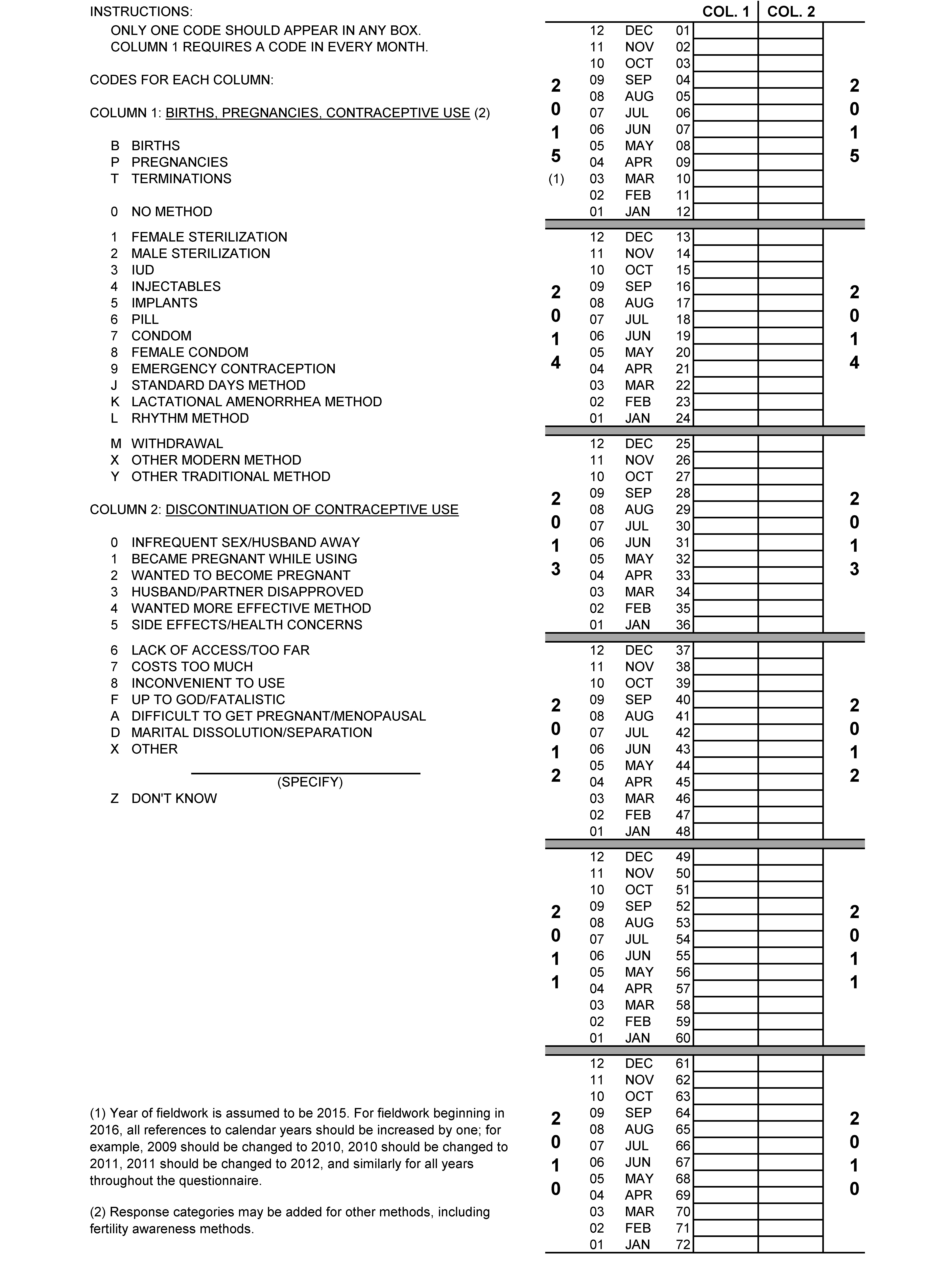
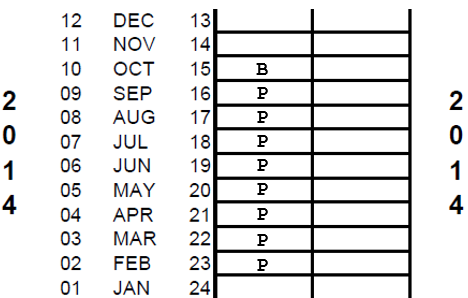
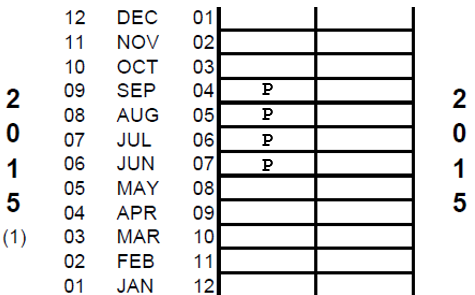
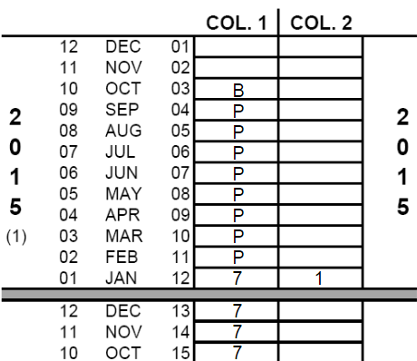
The possible response codes are those listed in the DHS-7 calendar. Only the main reason for discontinuation is recorded in column 2 in the row corresponding to the month the respondent stopped using the While filling in the episodes of contraceptive use in between each birth or pregnancy, any periods in which the respondent was neither pregnant nor using a contraceptive method are filled with code "0" meaning that no method was used in that month. After completing the data collection for the calendar, column 1 of the calendar will have a single code recorded in every row, except for those rows after the month of interview. Column 2 will have a single code in the same month as the month of discontinuation of each episode of contraceptive use. Other months in column 2 are left blank. For many respondents completing the calendar is quite straightforward. For example, a woman who has never been sexually active, a woman who used no contraception and had no pregnancies in the calendar period, or a woman who used the same contraceptive method throughout the calendar period (e.g. sterilization, IUD or Implant) would have the same code in all months of column 1 and no codes in column 2 of the calendar. Here is an example of a completed calendar. Briefly looking at the calendar, it is possible to read the reproductive and contraceptive events of this respondent. The example on the right shows a completed calendar of a respondent. At a first glance it is possible to know several pieces of information: Walking through the series of steps the interviewer goes through and using the DHS-7 calendar to interpret the codes, it is possible to see there are five categories of information we can read from this calendar: For more details on completing the calendar, watch the DHS program tutorial video on completing the calendar or see the DHS Interviewer’s manual.Example of a completed calendar
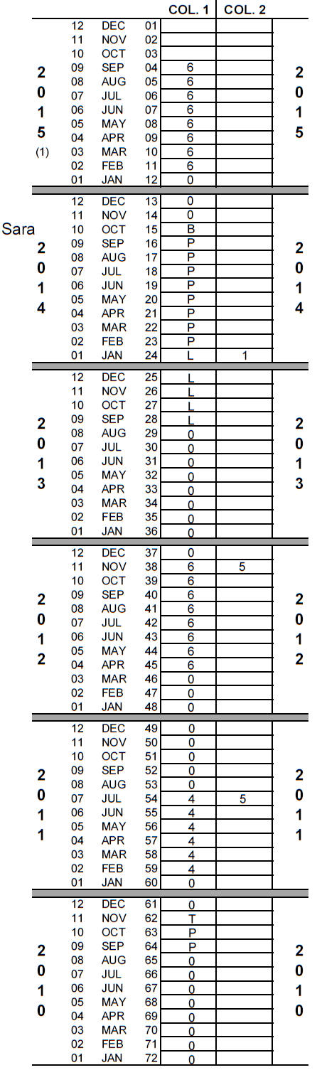
First Glance
Reproductive and Contraceptive Events
Birth in 2014 after 9 complete months of pregnancy.
The respondent is not currently pregnant.
One terminated pregnancy in November 2010 after three completed months of pregnancy.
The current method being used is the pill.
From 2010 to 2014, the respondent had several episodes of contraceptive use including using injectables, the pill, and the rhythm method (periodic abstinence). Her reasons for discontinuing these methods included side effects or health concerns and becoming pregnant while using.
Next section: 1.3 Uses of the calendar data
Module 1: What is the contraceptive (or reproductive) calendar?
Goal of the module: For analysts to understand what the DHS calendar is, its history, and how the data are collected.
1.3 Uses of the calendar data
The calendar provides information not collected in other parts of the DHS questionnaires. In particular the calendar is used to collect information on births and pregnancies, including pregnancy terminations (or non-live births) - miscarriages, abortions, and stillbirths. While the data on live births are also collected in the birth history3 (and are more readily analyzed using the birth history), the data on all non-live pregnancies in the calendar period are only collected in the calendar4. These data can be used to calculate pregnancy termination rates, including stillbirth rates, and, in conjunction with early neonatal mortality data, perinatal mortality rates.
Additionally, the calendar collects information on all episodes of contraceptive use and the reasons for discontinuation of each method used. The data can be used to understand contraceptive use dynamics, and particularly contraceptive discontinuation rates, failure rates and switching rates using lifetable analysis. Further, calendar data can be used to examine whether a contraceptive method was used before a birth or pregnancy, or if and when a woman started using a method in the postpartum period.
Below are a few examples of analyses that can be conducted with calendar data. Several of these are used as examples later in the tutorial:
| Analysis | Tutorial location |
|---|---|
| Method used prior to the most recent birth | Example 2 |
| Postpartum Family Planning: prevalence and method | Example 3 |
| Stillbirths and perinatal mortality | Example 4 |
| Reason for discontinuation of contraceptive method | Example 5, Example 8 |
| Contraceptive prevalence rate overtime, or at a specified time | Example 6 |
| Contraceptive use of any method in the prior n months | |
| Method switching in the prior n months | |
| Number of methods used in the five years preceding the interview | |
| Average duration of contraceptive use | |
| Average time to pregnancy after stopping use of a method | |
| Average time postpartum to starting use of contraception | |
| Contraceptive discontinuation, switching and failure rates | |
| Impact of contraceptive failure on unintended pregnancies |
3. The DHS data editing procedures attempt to ensure consistency of the information between the birth history and the calendar.
4. Except in surveys that use a full pregnancy history, rather than a birth history, in which case all non-live births are captured in the pregnancy history too.
Next section: 1.4 A brief history of the calendar
Module 1: What is the contraceptive (or reproductive) calendar?
Goal of the module: For analysts to understand what the DHS calendar is, its history, and how the data are collected.
1.4 A brief history of the calendar
1.4.1 History
The calendar was first developed for the DHS Program in the experimental surveys conducted in Peru and Dominican Republic in 1986. In particular, these surveys looked at “the potential of a six-year calendar for the collection of monthly data on contraceptive practice, breastfeeding, amenorrhea, postpartum abstinence and exposure to risk; the comparative merits of a calendar approach vs. the standard format of collecting such information within each birth interval for estimates of fecundability, natural fertility, and contraceptive efficacy;” (Peru Experimental Survey 1986).
Analysis of the data collected in the Peru survey showed improved information from the calendar format in the experimental questionnaire to the previously used tabular format. Goldman, Moreno and Westoff (1989) noted that “several different comparisons indicate that reporting of information on contraceptive histories in the experimental questionnaire is superior to that in the standard one.”
Moreno, Goldman and Babakol (1991) found other major advantages to using the calendar: “it obtains more complete reports of use for periods prior to the survey; it allows for a detailed study of contraceptive use patterns; and it obtains information which is more internally consistent with other types of information.”
On the basis of these experimental surveys and the analyses that followed, the use of the calendar became a standard part of the DHS Model A questionnaire for use in high contraceptive prevalence countries in the second phase of DHS (DHSII), starting in 1990.
1.4.2 Changes over time
| DHS Phases | Approximate years |
|---|---|
| I | 1984-89 |
| II | 1989-93 |
| III | 1993-97 |
| IV | 1997-03 |
| V | 2003-08 |
| VI | 2008-13 |
| 7 | 2013-18 |
Implementation of the DHS calendar has varied over survey phases. In phases II-IV, the calendar was included only in high contraceptive prevalence countries, which used the Model A questionnaire. In these phases, the calendar included columns that collected reasons for discontinuation (shown in Figure X), as well as a column tracking women’s marital/in-union status in each month of the calendar. Some calendars also included columns to capture additional information such as the source of contraception. Low contraceptive prevalence countries used the Model B questionnaire during phases II-IV, which did not include the calendar.
In DHS phase V starting in 2003, the use of separate questionnaires for high and low contraceptive prevalence countries was discontinued, and all countries used the same core questionnaire that included a calendar collecting births, pregnancies, terminations, and episodes of contraceptive use. Note that not all countries included the calendar in their questionnaires immediately. In some countries the calendar was not included until later phases of DHS, based on the data needs and interests of the country, sometimes preferring to maintain comparability with approaches used in prior surveys. Additionally, some countries adapted the calendar to collect only births, pregnancies, and terminations, excluding episodes of contraceptive use.
The current DHS-7 core questionnaire uses a two column calendar collecting month by month information on births, pregnancies and contraceptive use in column 1 and the reason for discontinuation in column 2, as pictured in Figure X. The DHSVI standard questionnaire followed the same format as in DHS-7. The DHSV standard questionnaire included only one column for births, pregnancies and contraceptive use, and did not include the reason for discontinuation of contraception; however countries that had previously used the calendar often included additional columns. Earlier rounds of the DHS questionnaires collected a variety of information in the calendar (see images below).
The calendar collects a complete history of women’s reproduction and contraceptive use6 for the calendar period prior to the survey. As noted earlier, the exact length of the period covered by the contraceptive calendar varies depending on the duration of data collection, whether the survey overlapped two years and the month in which the respondent was interviewed.
Table 2. Calendar columns in standard questionnaires
| Calendar columns in standard questionnaires | DHSII* | DHSIII* | DHSIV* | DHSV | DHSVI | DHS-7 |
|---|---|---|---|---|---|---|
| Births, pregnancies and contraceptive use | 1 | 1 | 1 | 1 | 1 | 1 |
| Reasons for discontinuation of contraception | 2 | 2 | 3 | 2 | 2 | |
| Source of contraception | 2 | |||||
| Duration of post-partum amenorrhea | 3 | |||||
| Duration of post-partum abstinence | 4 | |||||
| Duration of breastfeeding | 5 | |||||
| Marital/union status | 6 | 3 | 4 | |||
| Moves and types of communities | 7 | 4 | ||||
| Type of employment | 8 |
Some of the contraceptive methods used in column 1 of the calendar and their categorization have changed over time:
- In DHS I and II surveys, modern methods included pill, IUD, injection, vaginal methods, condom, female sterilization, and male sterilization. The vaginal methods included in a single group diaphragm, foam, and jelly. Traditional methods included periodic abstinence (of any kind), withdrawal, and all respondent- mentioned other methods.
- In DHS III surveys, modern methods included pill, IUD, injection, vaginal methods, condom, female sterilization, male sterilization, and implants. Traditional methods included periodic abstinence (of any kind), withdrawal, and lactational amenorrhea. Folk methods included respondent-mentioned other methods and were categorized separately from traditional methods.
- In DHS IV surveys, emergency contraception was added to the list of contraceptive methods but is not included as a separate method for current use (i.e., included in “other”). The questionnaire allowed for more than one method to be currently used but restricted the calendar to only one code (method) in each box according to the following hierarchy: female sterilization, male sterilization, contraceptive pill, intrauterine contraceptive device (IUD), contraceptive injection, contraceptive implants (Norplant), condoms, diaphragm, form or jelly, lactational amenorrhea method (LAM), periodic abstinence, withdrawal, and other methods.
- In DHS VI surveys, other modern method and other traditional methods were added to the list. Pill was moved after implants in the methods hierarchy. In DHS-7 surveys, emergency contraception and standard days method (SDM) are listed as separate methods; diaphragm and foam or jelly are included in “other modern method”.
Earlier versions of the DHS calendar can be found in:
DHSVI: www.dhsprogram.com/pubs/pdf/DHSQ6/DHS6_Questionnaires_5Nov2012_DHSQ6.pdf#page=89
The DHSVI calendar is the same as DHS-7.
DHSV: www.dhsprogram.com/pubs/pdf/DHSQ5/DHS5-Woman's-QRE-22-Aug-2008.pdf#page=63
The DHSV calendar is a single column calendar, the same as the first column for DHS-7.
DHSIV: www.dhsprogram.com/pubs/pdf/DHSQ4/DHS-IV-Model-A.pdf.pdf#page=110
The DHSIV calendar used 4 columns, with column 2 for sources of contraception, column 3 for reasons for discontinuation, and column 4 for marriage.
DHSIV: www.dhsprogram.com/pubs/pdf/DHSQ3/DHS-III-Model-A.pdf.pdf#page=90
The DHSIII calendar used 4 columns, with column 2 for reasons for discontinuation, column 3 for marriage, and column 4 for moves and types of communities.
DHSII: www.dhsprogram.com/pubs/pdf/DHSQ2/DHS-II-Model-A.pdf.pdf#page=87
The DHSII calendar used 8 columns: Column 1: Births, Pregnancies, and Contraceptive Use; Column 2: Discontinuation of Contraceptive Use; Column 3: Postpartum Amenorrhea; Column 4: Postpartum Abstinence; Column 5: Breastfeeding; Column 6: Marriage/Union; Colmun 7: Moves and Types of Communities; Column 8: Type of Employment.
1.4.3 Country-specific modifications
Various countries have made survey-specific modifications to the calendar to fit their data needs. These survey-specific modifications include the following:
Terminations and abortions: In certain surveys the terminated pregnancies are further classified as stillbirths, abortions or miscarriages. These surveys typically use a pregnancy history rather than a birth history in the women’s questionnaire. These data on the types of terminations are usually recorded in a survey-specific calendar variable.
Calendars with no method use: Some surveys used the calendar just to record births and terminated pregnancies, but not to record episodes of contraceptive use. In these surveys, the months of use or non-use of methods are left blank in the calendar.
Country-specific insertion and deletion of columns: Certain surveys have included additional columns in the calendar that are not typically part of the model questionnaire, or have removed standard columns from the questionnaire that are deemed less useful for the country.
Country-specific methods: All countries adapt the calendar to include the contraceptive methods that are appropriate and are in use in the country. The coding of the methods in the calendar follows the DHS standard recode format, but may include survey-specific codes for non-standard methods of contraception.
Non-western calendars: A few countries collect all of the data in the DHS questionnaire using a local calendar as the basis for all dates recorded in the questionnaire, and similarly as the basis for the DHS Contraceptive Calendar. To date these countries are:
- Ethiopia: The Ethiopian calendar is 7-8 years behind the Julian (Western) calendar, and the Ethiopian year starts around September 11th or 12th of each year (exact day varies). 1st July 2017 is 24 Sane (10) 2009 in the Ethiopian calendar. The Ethiopian calendar is made up of 12 months of 30 days, plus one month of 5 days (or 6 days in a leap year). The century month codes in the dataset are all based on the Ethiopian calendar, but squeezing the 13th month into a 12 month calendar. The start of the DHS calendar in the Ethiopian surveys is the first month of the Ethiopian year five years before the date of start of field work.
- Nepal: The Nepali calendar is 56-57 years ahead of the Julian (Western) calendar, and the Nepali year starts around mid-April of each year (exact day varies). 1st July 2017 is 17 Ashad (3) 2074 in the Nepali calendar. The Nepali calendar is made up of 12 months of between 28 and 32 days, and the number of days in a month can vary from year to year. The century month codes in the dataset are all based on the Nepali calendar. The start of the DHS calendar in the Nepali surveys is the first month of the Nepali year five years before the date of start of field work.
- Afghanistan: The Afghan calendar is 621-622 years behind the Julian (Western) calendar, and the Afghan year starts around March 20th or 21st of each year (exact day varies). 1st July 2017 is 10 Saratan (4) 1396 in the Afghan calendar. The Afghan calendar is made up of 12 months, the first 6 of which have 31 days, next 5 months have 30 days, and the last month has 29 or 30 days in a leap year. The century month codes in the dataset are all based on the Afghan calendar with 1300 as the base year, rather than 1900. The start of the DHS calendar in the Afghan surveys is the first month of the Afghan year five years before the date of start of field work.
Logic for handling survey-specific coding of the contraceptive methods and reasons for discontinuation are discussed in the section on survey-specific coding.
5. http://dhsprogram.com/publications/publication-FR32-Other-Final-Reports.cfm.
6. Some surveys in DHSV did not collect information on contraceptive use in the calendar period.
Next section: 1.5 Limitations of the calendar data
Module 1: What is the contraceptive (or reproductive) calendar?
Goal of the module: For analysts to understand what the DHS calendar is, its history, and how the data are collected.
1.5 Limitations of the calendar data
The DHS calendar data have some limitations that need to be kept in mind when analyzing the data. First and foremost, the calendar permits a single code to be captured for each individual month. This means that whenever two different events take place within a month, only one of them is recorded in that month. For example, if a respondent was using a contraceptive method at the beginning of the month, stopped using the method and switched to a different method in the same month then only one of these methods will be recorded for that month.
There is a hierarchy to the data collected in the calendar and the priority certain events have and this follows from the order in which the data are collected, as described in the prior section. The priority order for recording events in each month is as follows:
- 1) Live births
- 2) Completed months of pregnancy preceding live births
- 3) Months of current pregnancy
- 4) Terminated pregnancies
- 5) Completed months of pregnancy before a terminated pregnancy
- 6) Months of use of the current contraceptive method
- 7) Discontinuation of a contraceptive method, and months of use preceding the discontinuation
This has a number of implications, including:
- The calendar only permits a single code in each month, so cannot record any dual method use. For any women reporting using two methods concurrently, only one method is recorded and this is the first (generally the most effective) method from the list of method codes. In DHSV, DHSVI, and DHS-7 the list of methods were roughly ordered according to the effectiveness of the method.
- As for the contraceptive methods, the calendar does not permit reporting of more than one reason for discontinuation of a method. Respondents are asked for the main reason for discontinuation and this is recorded in the calendar.
- When switching methods, typically the method that was discontinued and the reason for discontinuation are recorded in that month, and the first month of use of the new method is recorded in the following month.
 If a respondent stops using a method in a month because they become pregnant, then either the method use or the pregnancy is recorded in the month. The months of pregnancy are recorded first, but because these are reported and recorded in completed months, typically the pregnancy would be recorded as starting in the following month, and the method will be recorded in the month in question.
For example, assume a respondent was using the condom until about 15th January 2015, when she became pregnant, and she gave birth around 15th October 2015 after 9 months of pregnancy. The interviewer would record a “B” in October 2015, and eight “P”s in September 2015 back to February 2015 (for a total of 9 months). The interviewer would also record the discontinuation of use of the condom in January 2015 together with the reason for discontinuation in column 2 of the calendar.
- If a delivery results in a live birth and a stillbirth in the same month then only the live birth is recorded in the calendar. This potentially results in a slight undercounting of stillbirths.
- For durations of pregnancy, respondents are asked for the number of completed months that they were pregnant, but we do not know this precisely. A birth in the calendar with a “B” and 8 “P”s is assumed to be a birth of 9 months gestation, but may be slightly shorter or longer.
- We also do not know the true duration of episodes of contraceptive use. The general rule is that completed months of pregnancy or completed months of use are recorded when durations are provided by the respondent. For example, if a respondent reported that she used a method for 8 months, we would see 8 boxes containing the code for that method.
- When respondents reported that they started use of a method in a particular month and stopped using it in a particular month, we don’t know when exactly that use started and stopped. For example, if we find that a respondent used the pill from February 2015 to April 2015 as marked in the calendar, this could be from February 1 to April 30 (3 months), or could be February 28 to April 1 (closer to 1 month). As mentioned above the general rule is that completed months of use are recorded in the calendar, but the imprecision of the calendar is a limitation.
In addition to these limitations, issues of quality of the data in the calendar are of concern, particularly recall bias. These are beyond the scope of this tutorial, but are discussed in “Contraceptive use and perinatal mortality in the DHS: an assessment of the quality and consistency of calendars and histories” (Bradley, Winfrey, and Croft 2015).
Next section: 2.1 How are the data stored in the calendar?
Module 2: How are the calendar data stored in datasets and how do I analyze the calendar data?
Goal of the module: For analysts to understand how the data are stored in the recode dataset.
2.1 How are calendar data stored in datasets?
The calendar represents the events in the year of interview up to the date of interview and the five (or, in several surveys, six) years preceding the year of interview (known as the calendar period). The calendar is split into up to 9 variables, representing each of up to 9 columns. Most surveys do not include all 9 columns, and many will have only 1 or 2 columns.
While the calendar is oriented vertically with the top of the calendar being the most recent point in time, the variables for the calendar are oriented horizontally, such that one column of the calendar is translated into one variable in the dataset. Each of the 9 variables contains a string of characters - one character for each month in the time period. The data are stored as single variables of 80 characters, allowing for up to 80 months to be represented in the calendar. The first character in each variable represents the most recent point in time, while the 80th character position represents data for January of the year in which the calendar started – January of the calendar year five years before the date of the start of the survey. The calendar variables are fixed at the 80th character position (January of the calendar year five years before the start of the survey), such that the first few positions in the calendar strings represent points in time after the date of interview, and are consequently left blank.
The variables for the calendar are the series of VCAL variables, named differently in the different software to follow software specific naming conventions:
| Col. | Stata | SPSS | SAS | Contents |
|---|---|---|---|---|
| 1 | vcal_1 | VCAL$1 | VCAL_1 | Births, pregnancies, and contraceptive use |
| 2 | vcal_2 | VCAL$2 | VCAL_2 | Reason for discontinuation of contraceptive use |
| 3 | vcal_3 | VCAL$3 | VCAL_3 | Marital/union status (vcal_6 in DHSII recode files) |
| 4 | vcal_4 | VCAL$4 | VCAL_4 | Moves and types of communities (vcal_7 in DHSII recode files) |
| 5 | vcal_5 | VCAL$5 | VCAL_5 | Source of contraception |
| 6 | vcal_6 | VCAL$6 | VCAL_6 | Survey-specific |
| 7 | vcal_7 | VCAL$7 | VCAL_7 | Survey-specific |
| 8 | vcal_8 | VCAL$8 | VCAL_8 | Survey-specific |
| 9 | vcal_9 | VCAL$9 | VCAL_9 | Survey-specific |
In most references from here on, the calendar variables will be referenced only by the Stata variable names, e.g. vcal_1, except in the examples where the appropriate name within the software is used.
The variables in the recode files are recoded to follow this standard ordering convention, which may not be the ordering of columns that was used in the survey questionnaire. Note that this standard ordering convention has been in use since DHSIII surveys onwards, but in DHSII surveys there were eight standard columns, following the standard ordering of the calendar columns in the model questionnaire at that time, plus one survey-specific calendar variable.
The codes used in each of the calendar variables also follow a standard coding scheme, not the coding scheme used in the survey questionnaire. Note that while the DHS-7 core questionnaire only includes two columns, the DHS recode file allows for five standard calendar variables and four survey-specific calendar variables. The standard coding scheme for the additional standard variables is used in surveys in countries that opted to collect this additional information. The codes for each standard column are given below:
Table 3. Standard coding scheme used in recode files (R) and standard DHS-7 questionnaires (Q)
| R | Q | vcal_1 (Pregnancies and contraception) | R | Q | vcal_2 (Reasons for discontinuation) | R | Q | vcal_3 (Marriage) |
|---|---|---|---|---|---|---|---|---|
| B | B | Birth | X | In union (married or living together) | ||||
| T | T | Terminated pregnancy/non-live birth | 0 | Not in union | ||||
| P | P | Pregnancy | vcal_4 (Residence) | |||||
| 0 | 0 | Non-use of contraception | X | Change of community | ||||
| 1 | 6 | Pill | 1 | 1 | Became pregnant while using | 0 | Capital/Major city (country-specific) | |
| 2 | 3 | IUD | 2 | 2 | Wanted to become pregnant | 1 | City | |
| 3 | 4 | Injectables | 3 | 3 | Husband disapproved | 2 | Town | |
| 4 | Diaphragm | 4 | 5 | Side effects/health concerns | 3 | Countryside | ||
| 5 | 7 | Condom | 5 | Health concerns3 | 4 | Abroad (country-specific) | ||
| 6 | 1 | Female sterilization | 6 | 6 | Access/availability | ? | Missing data for type of residence | |
| 7 | 2 | Male sterilization | 7 | 4 | Wanted a more effective method | vcal_5 (Source of contraception) | ||
| 8 | L | Periodic abstinence/rhythm | 8 | 8 | Inconvenient to use | Country-specific | ||
| 9 | M | Withdrawal | 9 | Infrequent sex/husband away | ||||
| W | Y | Other traditional methods | C | 7 | Cost too much | |||
| N | 5 | Implants | F | F | Up to God/fatalistic | |||
| A | Abstinence | A | A | Difficult to get pregnant/menopausal | ||||
| L | K | Lactational amenorrhea method (LAM) | D | D | Marital dissolution/separation | |||
| C | 8 | Female condom | W | X | Other | |||
| F | Foam and Jelly | K | Z | Don't know | ||||
| E1 | 9 | Emergency contraception (DHSVI) | ||||||
| S1 | J | Standard days method (DHSVI) | ||||||
| M1 | X | Other modern method (DHSVI) | ||||||
| α2 | Country-specific method 1 | α2 | Country-specific reason 1 | |||||
| ß2 | Country-specific method 2 | ß2 | Country-specific reason 2 | |||||
| τ2 | Country-specific method 3 | τ2 | Country-specific reason 3 | |||||
| ? | ? | Unknown method/missing data | ? | ? | Missing |
1 letters E, S, and M were added as standard codes in DHSVI and DHS-7, however these codes may have been used for other survey-specific methods in earlier phases of DHS
2 α, ß, τ are place-holders and are replaced by survey-specific letters – see Calendar recoding.do or Calendar recoding.sps for the meaning of the survey-specific codes.
3 Used separately in earlier phases of DHS, but combined with code 4 in later phases.
Rows in the calendar representing months after the month of interview are left blank. With this exception, when the columns are used, variables vcal_1, vcal_3 and vcal_4 do not contain any blank characters.
How can I understand the calendar?
The calendar data are stored in the datasets in reverse chronological order with the left hand end of the calendar string variables referring to dates near the date of interview and the right hand end of the string referring to dates five years before the date of interview. In discussing the contents of the calendar it is often useful to read the calendar data from right to left. The right hand end of the calendar, in position 80 of each string, represents January of the calendar year five years prior to the start of the survey. In this example the calendar starts January 2010, with the year of start of survey being 2015.
Below is an example of a calendar in the recode dataset:
Year      | <-2016-><---2015---><---2014---><---2013---><---2012---><---2011---><---2010--->
Month     | AJJMAMFJDNOSAJJMAMFJDNOSAJJMAMFJDNOSAJJMAMFJDNOSAJJMAMFJDNOSAJJMAMFJDNOSAJJMAMFJ
____________________________________________________________________________________________
vcal_1    |            11111111000BPPPPPPPP88888000000000111111110000000033333300TPP00000000
vcal_2    |                                1             4               5
vcal_3    |            XXXXXXXXXXXXXXXXXXXXXXXXXXXXXXXXXXXXXXXXXXXXXXXXXXXXXXXXXXXXXXXXX0000
vcal_4    |            0000000000000000000000000000X1111111111111111111111111111X33333333333
vcal_5    |                   2                F                2             3
____________________________________________________________________________________________
Position  | ....5...10...15...20...25...30...35...40...45...50...55...60...65...70...75...80
vcal_1 through vcal_5 in their dataset. “Position” refers to the character position in the character string variable representing each column of the calendar. Position 1 is the first character, and position 80 is the last character of the string variables.
The example above uses the same information as in the example of a completed calendar for the first two columns of the calendar (vcal_1 and vcal_2) and adds example data for marriage (vcal_3), moves and types of places of residence (vcal_4), and sources of contraception (vcal_5).
In the above example, reading from the right hand end of the calendar strings:
- In January 2010 (position 80), the respondent was not using any method of contraception (
vcal_1= 0), was not married (vcal_3= 0), was living in the countryside (vcal_4= 3). - In May 2010 the respondent was married (
vcal_3position 76 = X). - In September 2010 the respondent became pregnant (
vcal_1position 72 = P) and the pregnancy lasted 3 months and resulted in a terminated pregnancy in November 2010 (vcal_1position 70 = T). - In December 2010 the respondent moved from the countryside to a city (
vcal_4position 69 = X, position 68 = 1). - Two months later in February 2011 the respondent started using Injectable as a contraceptive method (
vcal_1position 67 = 3), after she got the method from a family planning clinic (vcal_5position 67 = 3). - She used the Injectable until July 2011 (
vcal_1position 62 = 3, position 61 = 0) when she stopped using the method as she had health concerns about the method (vcal_2position 62 = 5). - She did not use any method until April 2012 when she started using the Pill (
vcal_1position 53 = 1), which she got from a government health center (vcal_5position 53 = 2). - She used the Pill until November 2012 (
vcal_1position 46 = 1, position 45 = 0) when she stopped because of side effects (vcal_2position 46 = 4). - The respondent moved again in May 2013, this time to the capital city (
vcal_4position 40 = X, position 39 = 0). - In September 2013 the respondent start using Periodic Abstinence (or Rhythm method) (
vcal_1position 36 = 8), a method she learned about from a friend or relative (vcal_5position 36 = F). - She used Periodic Abstinence until January 2014 (
vcal_1position 32 = 8, position 31 = P) when she discontinued because she became pregnant (vcal_2position 32 = 1). - The pregnancy continued up to October 2014 when she gave birth to a child (
vcal_1position 23 = B). - Following the birth of the child the respondent started using the Pill in February 2015 (
vcal_1position 19 = 1). She acquired the method from a government health center (vcal_5position 19 = 2). - The respondent continued using the Pill until the interview (
vcal_1position 12 = 1).
Months in the calendar after the month of interview are filled with blank spaces (positions 1-11) in each calendar variable.
For more information, watch the DHS Program tutorial video on the data structure of the contraceptive calendar.
Supplementary variables used with the calendar
There are four additional variables that are invaluable in using the calendar:
v017Century month code (CMC)7 for the first month of the calendar. This is constant for all cases and is the century month code of January of the year five years before the start of the survey.v018Row of calendar representing the month of interview. The calendar is numbered from 1 to 80, with month 80 being January of the first year of the calendar, and the month of interview typically in rows 1 to 20.v019Records the length of the calendar to use for this case.v019is equal to80-v018+1. Typically the values are in the range of 60-80.v019aNumber of calendar columns used in this dataset.
These variables will be used in the examples to facilitate the processing of the calendar.
In the example given above:
v017= 1321 = ((2010-1900)*12+1)v018= 12 (equivalent to September 2015 in the example)v019= 69 (the length of the used part of the calendar invcal_1)v019a= 5 (asvcal_1throughvcal_5are used)
7. The century month code is the number of months since the beginning of 1900 and is calculated as CMC = (YYYY – 1900)*12 + MM, where YYYY is the year and MM is the month.
Next section: 2.2 Analyzing the calendar data in statistical software
Module 2: How are the calendar data stored in datasets and how do I analyze the calendar data?
Goal of the module: For analysts to understand how the data are stored in the recode dataset.
2.2 Analyzing the calendar data in statistical software
There are three basic approaches to processing the data in the calendar:
- String parsing of the calendar (Module 3).
- Reshaping or restructuring the calendar into a file of single months (Module 4).
- Reshaping or restructuring the calendar into event files (Module 5).
Each of these approaches has advantages for different types of analysis. The string manipulation approach described in Module 3, does not require restructuring or reshaping the data, but does require stronger skills with the use of the string functions which we demonstrate with multiple examples. It can be a useful approach when analyzing a series of events, e.g. use of a contraceptive method following a birth. This approach is often useful when the unit of analysis is the woman and restructuring of the data is not required.
The second approach described in Module 4, restructuring the calendar into a file of single months, while conceptually simpler, does not provide as much flexibility for analysis. This approach is useful when the unit of analysis is something other than the woman, and can work well when reference to prior or following events in the calendar is not necessary.
The use of event files as described in Module 5, provides a combination of the two prior approaches, and permits more complex analyses of the data. The event file approach is particularly useful when the unit of analysis is something other than the woman, e.g. births, pregnancies, episodes of contraceptive use or non-use. Once event files are constructed, these are often simpler to use in analyses.
For all approaches some string manipulation functions are needed to handle the data, either in restructuring the data or in the analysis of the data. Additionally the concept of looping is used in the manipulation of the calendar data to "loop" through each of the months in the calendar.
In the following modules, examples are shown for use in Stata and SPSS. Logic for Example 1 also exists for SAS, R, CSPro and Excel. Logic for all examples can be found in the Programs and coding resources: Examples files. Output is presented following the logic for each example where there is useful output, and is only presented for Stata for brevity. In many cases the output for a particular step is just a repetition of the commands and is not shown in this document. Output files for each example are available in the Programs and coding resources: Examples files for each software.
The examples that follow use the DHS Model Datasets, based on the standard DHS Individual Recode, but can be applied to any of the DHS survey datasets. However, every survey dataset has survey-specific differences and some of these can affect the calendar data. See the section on survey-specific coding for more details of these differences.
Next section: 3.1 String functions
Module 3: String parsing of the calendar
Goal of the module: For analysts to understand how to use string manipulation functions to access the data.
3.1 String functions
To read the data in the calendar and extract information from the calendar, a number of string functions in the appropriate statistical software are needed. These functions are needed to extract portions of the calendar strings (substring functions), calculate the length of strings (length functions), find particular codes in the calendar strings (position functions), remove leading or trailing blanks from strings (trimming functions), reverse strings to analyze them in the opposite order (reversal functions). A list of useful functions is provided below and are demonstrated in Example 1.
In the below function descriptions, str is usually the calendar string variable (e.g. vcal_1/VCAL$1/VCAL_1) or a portion of it. Useful functions in each of the software include the following:
| Length of a string | strlen(str) |
| Position in string | strpos(str,str1) - the position in str at which str1 is first found |
| Substring | substr(str,pos,len) - the substring of str, starting at pos, for a length of len |
| Reverse a string | reverse(str) |
| Remove blanks | trim(str) – leading and trailing blanksltrim(str) – leading blanksrtrim(str) – trailing blanks |
| Other useful string functions | indexnot(str,str1) – returns position of first character in str not found in str1subinstr(str,str1,str2,n) – substitutes str1 with str2 in str up to n times |
| Other useful functions | inrange(val,min,max) – if val is between min and maxinlist(val,val1,val2,val3,...) – if code>val is equal to one of val1, val2, val3, etc. |
| Length of a string | char.length(str) |
| Position in string | char.index(str,str1) - the position in str at which str1 is first found |
| Substring | char.substr(str,pos,len) - the substring of str, starting at pos, for a length of len |
| Reverse a string | See user macro !ReverseStr in Example1.sps:
define !ReverseStr(!positional !tokens(1) /!positional !tokens(1))
* first parameter is old variable, second is new variable.
compute !2 = !1.
string #a (A1).
compute #l = length(rtrim(!2)).
loop #i = 1 to #l/2.
+ compute #j = #l - #i + 1.
+ compute #a = char.substr(!2,#i,1).
+ compute substr(!2,#i,1) = char.substr(!2,#j,1).
+ compute substr(!2,#j,1) = #a.
end loop.
execute.
!enddefine.

string rev_cal (a80).
* reverse vcal$1 into rev_cal.
!ReverseStr vcal$1 rev_cal
|
| Remove blanks | rtrim(str) – trailing blanksltrim(str) – leading blanks |
| Other useful string functions | string(num) – converts a number to a stringnumber(str) – converts a string to a number |
| Length of a string | length(str) |
| Position in string | index(str,str1) |
| Substring | substr(str,pos,len) |
| Reverse a string | reverse(str) |
| Remove blanks | strip(str) |
| Length of a string | nchar(str) |
| Position in string | regexr(str1,str,fixed=TRUE) |
| Substring | substr(str,start,stop) |
| Reverse a string | strReverse <- function(x) {
sapply(lapply( strsplit(x, NULL), rev), paste, collapse="")
return(x)
}
strReverse(str) |
| Remove blanks | trim <- function (x) {
gsub("^\\s+|\\s+$", "", x)
return(x)
}
trim(str) |
| Length of a string | length(str) |
| Position in string | pos(str1,str) |
| Substring | str[pos:len] |
| Reverse a string | See user function reverseStr(str) in Example1.bch.apc:
function string reverseStr(string str);
  string c;
  numeric l = length(str);
  numeric i, j;
  do i = 1 while i <= l/2
    j = l-i+1;
    c = str[i:1];
    str[i:1] = str[j:1];
    str[j:1] = c;
  enddo;
  reverseStr = str;
end;

reverseStr(str)
|
| Remove blanks | strip(str) - trailing blanksSee user function ltrim(str) in Example1.bch.apc:
function string ltrim(string str)
  numeric i;
  do i = 1 while i <= length(str) & str[i:1] = " "; enddo;
  ltrim = str[i:length(str)-i+1];
end;

ltrim(str)
- leading blanks |
| Length of a string | len(str) |
| Position in string | iferror(find(str1,str),0) |
| Substring | mid(str,pos,len) |
| Reverse a string | Use a VBA macro with the function StrReverse(str), as follows:Function ReverseStr(str As String) As String |
| Remove blanks | trim(str) – leading and trailing blanksltrim(str) – leading blanksrtrim(str) – trailing blanks |
| Stata | SPSS | SAS | R | CSPro | Excel | |
|---|---|---|---|---|---|---|
| Length of a string | strlen(str) | char.length (str) | length(str) | nchar(str) | length(str) | len(str) |
| Position in string | strpos(str, str1) | char.index(str,str1) | index(str,str1) | regexpr(str1, str, | pos(str1, str) | iferror( find |
| Substring | substr(str,pos,len) | substr(str,pos,len) | substr(str,pos,len) | substr(str,start,stop) | str[start:len] | mid(str,pos, len) |
| Reverse a string | reverse(str) | SPSS user-defined macro | reverse(str) | strReverse <- | CSPro user-defined function | Excel macro |
| Removing blanks | trim(str)(leading and trailing - see also ltrim and rtrim) | rtrim(str)(trailing blanks - see also ltrim) | strip(str)(leading and trailing - see also left and trim) | trim <- | strip(str)(removes trailing blanks only) | trim(str)(leading and trailing - see also ltrim and rtrim) |
Next section: 3.2 Example data
Module 3: String parsing of the calendar
Goal of the module: For analysts to understand how to use string manipulation functions to access the data.
3.2 Example data
All of the examples assume that the data and programs are stored in C:\Data\DHS_model\, and are designed to work with the DHS model dataset for the individual (women's) recode file appropriate for the software. Change the appropriate command in each example file if the dataset is stored in a different folder. The examples assume that the following model datasets are being used:
- Stata:zzir62fl.dta (Stata dataset)
- SPSS: zzir62fl.sav (SPSS dataset)
- SAS: zzir62fl.sd2 (SAS dataset)
- R: zzir62fl.dta (Stata dataset)
- CSPro:zzir62.dat (Hierarchical file)
- Excel:The Excel example uses vcal_1 copied from zzir62fl.dta and pasted into Excel
Next section: Example 1 - Basic string functions
Module 3: String parsing of the calendar
Goal of the module: For analysts to understand how to use string manipulation functions to access the data.
Example 1 - Basic string functions
The first example demonstrates how some of the basic string functions work and the output that they give. Examples are given for some of the basic string functions for several different software:
- 1. Displaying the first column of the calendar for a few respondents
- 2. Calculating the full length of the calendar
- 3. Extracting a substring from the calendar, starting in position 44 and extracting 12 characters
- 4. Finding the position in the calendar of the first occurrence of letter "P"
- 5. Reversing the calendar
- 6. Trimming the calendar to remove leading and trailing blanks
- 7. Calculating the length of the calendar actually used for a case
For each example, it is useful to remember that the data shown are in reverse chronological order with the left hand end of the string being nearest to the date of interview and the right hand end of the string representing the beginning of the calendar five years prior to the year of the start of the survey.
Logic for example 1 can be found in the following files:
| Software | Commands | Output |
|---|---|---|
| Stata | Stata\Example1.do | Stata\Example1.log |
| SPSS | SPSS\Example1.sps | SPSS\Example1.txt |
| SAS | SAS\Example1.sas | SAS\Example1.pdf |
| R | R\Example1.R | R\Example1.txt |
| CSPro | CSPro\Example1.bch.apc | CSPro\Example1.lst |
| Excel | Excel\Example1.xls | |
E1.1Displaying the first column of the calendar for a few respondents
Let us start by displaying the calendar data from the first column (vcal_1/VCAL$1) for the first few cases in the dataset, just to see what the calendar data look like.
* DHS Calendar Tutorial - Example 1
* Basic string manipulation

* download the model dataset for individual women's recode: "ZZIR62FL.DTA"
* the model datasets are available at http://dhsprogram.com/data/download-model-datasets.cfm

* change to a working directory where the data are stored
* or add the full path to the 'use' command below
cd "C:\Data\DHS_model"

* open the dataset, selecting just the variables we are going to use
use vcal_1 v000 v005 v007 v008 v017 v018 v019 using "ZZIR62FL.DTA", clear

* 1) display column 1 of the calendar for the first 6 respondents
list vcal_1 in 1/5
* DHS Calendar Tutorial - Example 1.
* Basic string manipulation.

* download the model dataset for individual women's recode: "ZZIR62FL.SAV"
* the model datasets are available at http://dhsprogram.com/data/download-model-datasets.cfm .

* change to a working directory where the data are stored
* or add the full path to the 'get file' command below.
cd "C:\Data\DHS_model".

* open the dataset, and just keep the variables we are going to use.
get file="ZZIR62FL.SAV" / keep vcal$1 v000 v005 v007 v008 v017 v018 v019.

* 1) display column 1 of the calendar for the first 6 respondents.
list variables = vcal$1 /cases from 1 to 5.
. * 1) display column 1 of the calendar for the first 6 respondents
. list vcal_1 in 1/5

     +----------------------------------------------------------------------------------+
     |                                                                           vcal_1 |
     |----------------------------------------------------------------------------------|
  1. |               00000BPPPPPPPP00000000000000000000000BPPPPPPPP00000000000000000000 |
  2. |               PPPPPP000000000000000000000000BPPPPPPPP000000000000000000000000000 |
  3. |               000000000000000000000000000000000000000000000000000000000000000000 |
  4. |               0000000000BPPPPPPPP00000000000BPPPPPPPP000000000000000000000000000 |
  5. |               0BPPPPPPPP000000000000000000000000BPPPPPPPP00000000000000000000000 |
     +----------------------------------------------------------------------------------+
E1.2Calculating the length of the calendar
Let us next check how long the calendar strings are. In the standard individual recode format, the calendar strings are 80 characters long, but we can confirm that by calculating the length. The function strlen (in Stata) or char.length (in SPSS) will return the length of the calendar string.
* 2) calculate the full length of calendar by displaying length of strings
gen vcal_len = strlen(vcal_1)
label variable vcal_len "length of calendar"
list vcal_len in 1/5
* 2) calculate the full length of calendar by displaying length of strings.
compute vcal_len = char.length(vcal$1).
variable labels vcal_len "Length of calendar".
print formats vcal_len (F2.0).
list variables = vcal_len /cases from 1 to 5.
. * 2) calculate the full length of calendar by displaying length of strings
. gen vcal_len = strlen(vcal_1)

. label variable vcal_len "length of calendar"

. list vcal_len in 1/5

     +----------+
     | vcal_len |
     |----------|
  1. |       80 |
  2. |       80 |
  3. |       80 |
  4. |       80 |
  5. |       80 |
     +----------+
E1.3Extracting a substring from the calendar
Let us say that we want to look at a particular part of the calendar, say, a year prior to or following a particular date, and for this example let us use the 12-month window from position 44-55 of the calendar.
In Stata we can use the substr function to extract a piece of a substring. In SPSS we use the char.substr function, but we must remember to define the string variable (string piece (A12).) we are putting the piece of the string into, and make sure it is big enough to hold the string.
* 3) take a piece of a string from column 1
gen piece = substr(vcal_1,44,12) // start at position 44 for 12 characters
label variable piece "piece of calendar"
list piece in 1/5
* 3) take a piece of a string from column 1.
string piece (A12).
compute piece = char.substr(vcal$1,44,12).
variable labels piece "Piece of calendar".
print formats piece (A12).
list variables = piece /cases from 1 to 5.
. * 3) take a piece of a string from column 1
. gen piece = substr(vcal_1,44,12) // start at position 44 for 12 characters

. label variable piece "piece of calendar"

. list piece in 1/5

     +--------------+
     |        piece |
     |--------------|
  1. | 00000000BPPP |
  2. | 0BPPPPPPPP00 |
  3. | 000000000000 |
  4. | 0BPPPPPPPP00 |
  5. | 00000BPPPPPP |
     +--------------+
Often we will this method of extraction just to capture a single character from the calendar, representing a single month, for example to capture the type of contraceptive method used in a particular month x using either substr(vcal_1,x,1) or char.substr(vcal$1,x,1).
E1.4Finding the position in the calendar of the first occurrence of letter "P"
We can use the strpos (Stata) or char.index (SPSS) functions to find the position in the calendar string where something happens, such as a birth, a month of pregnancy, or the use or non-use of contraception. In the below example, we look for the last use of the letter "P" in the calendar (i.e. nearest to the date of interview). This may be because the woman is currently pregnant, but could also be the last month of pregnancy before the month in which the birth of a child or a pregnancy termination took place.
* 4) find the position of a substring within a string
gen pos = strpos(vcal_1,"P") // look for first occurrence of "P"
label variable pos "position in calendar"
list pos in 1/5
* 4) find the position of a substring within a string.
compute pos = char.index(vcal$1,"P").
variable labels pos "Position in calendar".
print formats pos (F2.0).
list variables = pos /cases from 1 to 5.
. * 4) find the position of a substring within a string
. gen pos = strpos(vcal_1,"P") // look for first occurrence of "P"

. label variable pos "position in calendar"

. list pos in 1/5

     +-----+
     | pos |
     |-----|
  1. |  21 |
  2. |  15 |
  3. |   0 |
  4. |  26 |
  5. |  17 |
     +-----+
E1.5Reversing the calendar
The calendar is organized with the most recent point in time at the beginning of the string and the point furthest back in time at the end of the string. Sometimes, though, it is easier to work with the calendar in the opposite order with the first position being the furthest back in time and the last positions being the most recent. This can be achieved by reversing the calendar string. In Stata there is a function reverse to do just this, however, in SPSS no equivalent exists. Instead, we can write a macro that achieves the same thing. In the SPSS logic below, we define a macro called !ReverseStr that will reverse a string, and then use that macro in the logic below.
* 5) reverse a string
gen rev_cal = reverse(vcal_1) // calendar from oldest to most recent month (L to R)
label variable rev_cal "reversed calendar"
list rev_cal in 1/5
* 5) reverse a string
* macro to reverse a string.
define !ReverseStr(!positional !tokens(1) /!positional !tokens(1))
* first parameter is old variable, second is new variable.
compute !2 = !1.
string #a (A1).
compute #l = length(rtrim(!2)).
loop #i = 1 to #l/2.
+ compute #j = #l - #i + 1.
+ compute #a = char.substr(!2,#i,1).
+ compute substr(!2,#i,1) = char.substr(!2,#j,1).
+ compute substr(!2,#j,1) = #a.
end loop.
execute.
!enddefine.

* reverse a string.
string rev_cal (a80).
* reverse vcal$1 into rev_cal.
!ReverseStr vcal$1 rev_cal
variable labels rev_cal "Reversed calendar".
print formats rev_cal (A80).
list variables = rev_cal /cases from 1 to 5.
. * 5) reverse a string
. gen rev_cal = reverse(vcal_1) // calendar from oldest to most recent month (L to R)

. label variable rev_cal "reversed calendar"

. list rev_cal in 1/5

     +----------------------------------------------------------------------------------+
     |                                                                          rev_cal |
     |----------------------------------------------------------------------------------|
  1. | 00000000000000000000PPPPPPPPB00000000000000000000000PPPPPPPPB00000               |
  2. | 000000000000000000000000000PPPPPPPPB000000000000000000000000PPPPPP               |
  3. | 000000000000000000000000000000000000000000000000000000000000000000               |
  4. | 000000000000000000000000000PPPPPPPPB00000000000PPPPPPPPB0000000000               |
  5. | 00000000000000000000000PPPPPPPPB000000000000000000000000PPPPPPPPB0               |
     +----------------------------------------------------------------------------------+
E1.6Trimming the calendar to remove leading and trailing blanks
It is sometimes useful to trim a string to exclude blanks from the beginning or end (or both) of a string, for example, if we wanted to remove the empty months after the date of interview from the beginning of the calendar. Functions ltrim and rtrim can be used in both Stata and SPSS, and Stata also includes just trim that removes blanks from both ends of a string. In SPSS we need to use a combination of ltrim and rtrim to do the same.
* 6) trim a string of leading and trailing spaces
gen trim_cal = trim(vcal_1)
label variable trim_cal "trimmed calendar"
list trim_cal in 1/5
* 6) trim a string of leading and trailing spaces.
string trim_cal (a80).
compute trim_cal = rtrim(ltrim(vcal$1)).
variable labels trim_cal "Trimmed calendar".
print formats trim_cal (A80).
list variables = trim_cal /cases from 1 to 5.
. * 6) trim a string of leading and trailing spaces
. gen trim_cal = trim(vcal_1)

. label variable trim_cal "trimmed calendar"

. list trim_cal in 1/5

     +--------------------------------------------------------------------+
     |                                                           trim_cal |
     |--------------------------------------------------------------------|
  1. | 00000BPPPPPPPP00000000000000000000000BPPPPPPPP00000000000000000000 |
  2. | PPPPPP000000000000000000000000BPPPPPPPP000000000000000000000000000 |
  3. | 000000000000000000000000000000000000000000000000000000000000000000 |
  4. | 0000000000BPPPPPPPP00000000000BPPPPPPPP000000000000000000000000000 |
  5. | 0BPPPPPPPP000000000000000000000000BPPPPPPPP00000000000000000000000 |
     +--------------------------------------------------------------------+
E1.7Calculating the length of the calendar actually used
Finally, we can calculate the length of the calendar that is actually used, dropping the months after the date of interview. We can do this by calculating the length of the trimmed calendar.
* 7) display the length of calendar actually used, from the trimmed version
gen vcal_used = strlen(trim_cal)
label variable vcal_used "length of calendar used"
* should be the same as v019
list vcal_used v019 in 1/5
* 7) display the length of calendar actually used, from the trimmed version.
compute vcal_used = char.length(trim_cal).
variable labels vcal_used "Length of calendar used".
print formats vcal_used (F2.0).
* should be the same as v019.
list variables = vcal_used v019 /cases from 1 to 5.
. * 7) display the length of calendar actually used, from the trimmed version
. gen vcal_used = strlen(trim_cal)

. label variable vcal_used "length of calendar used"

. * should be the same as v019
. list vcal_used v019 in 1/5

     +-----------------+
     | vcal_u~d   v019 |
     |-----------------|
  1. |       66     66 |
  2. |       66     66 |
  3. |       66     66 |
  4. |       66     66 |
  5. |       66     66 |
     +-----------------+
These are just a few of the most useful string parsing functions that can be used, but are the ones that are used most commonly in processing the calendar data.
Next section: Example 2 - Last pregnancy, duration of pregnancy and method used before pregnancy
Module 3: String parsing of the calendar
Goal of the module: For analysts to understand how to use string manipulation functions to access the data.
Example 2 - Last pregnancy, duration of pregnancy and method used before pregnancy
For this next example, we are interested in looking at contraceptive use prior to the last birth or terminated pregnancy. We will use this example to find the last live birth or terminated pregnancy in the calendar, and then look for contraceptive use prior to that pregnancy, and can then compare contraceptive use or non-use prior to a live birth or a terminated pregnancy.
- 0. Open the dataset and set up the data
- Example 2A – Find the century month code (CMC) of the last pregnancy in the calendar
- 1. Get the length of the calendar
- 2. Find the position of the last birth or terminated pregnancy in the calendar
- 3. Calculate the century month code (CMC) of the last pregnancy in the calendar
- Example 2B – Find the duration of pregnancy for the last pregnancy
- 4. Calculate the duration of the pregnancy and find the position of the month before the pregnancy for the last pregnancy
- Example 2C - Check if a contraceptive method was used at some time before the pregnancy, but in the 5 years preceding the survey, and find the method
- 5. Find the last month before the pregnancy but within the last 5 years that the respondent has a code different from 0 (something other than non-use of contraception), and
- 6. Check if the respondent used a method at that time
- 7. Convert the alphanumeric string variable for the method to a numeric code
- 8. Label the method variable and codes
- 9. Weight and tabulate the method used by type of pregnancy
Logic for example 2 can be found in the following files:
| Software | Commands | Output |
|---|---|---|
| Stata | Stata\Example2.do | Stata\Example2.log |
| SPSS | SPSS\Example2.sps | SPSS\Example2.txt |
As mentioned before, remember that the calendar is stored in reverse chronological order and the left hand end of a string represents a more recent time point than the right hand end of the string. Example 1 demonstrated the use of functions to return the length of a string, search a string and find the position of an event in the string, capture the code at a particular position in the string, and create substrings to carry out the steps laid out above. In Example 2, the logic looks for the last birth or terminated pregnancy, then the month before the pregnancy, and then the last month of use of contraception progressing from left (more recent) to right (further back in time) through the calendar.
Example:
if calendar is as below ("_" used to replace blanks for months after the date of interview for display here):
______________00000BPPPPPPPP000000555555500000TPP00000000000000BPPPPPPPP00000000
1)	Length is 80 characters
2)	Position of last birth or terminated pregnancy is position 20. Pregnancy resulted in a live birth.
______________00000BPPPPPPPP000000555555500000TPP00000000000000BPPPPPPPP00000000
                   ^
3)	Century month code is 1381 (assuming interview in CMC 1386 [position 15])
4)	Duration of pregnancy is 9 months and position of month before pregnancy is position 29
______________00000BPPPPPPPP000000555555500000TPP00000000000000BPPPPPPPP00000000
                   |12345678^
5)	Last month with a code other than 0 before pregnancy is in position 35
______________00000BPPPPPPPP000000555555500000TPP00000000000000BPPPPPPPP00000000
                                  ^
6)	Respondent was using a method, method code “5” (Condom)
7)	Numeric version of the method code is 5
E2.0Open the dataset and set up the data
The examples below assume the data are in C:\Data\DHS_model\, and that the dataset being used is ZZIR62FL.DTA. Adjust the filename and the folder name to match the file you are using and the folder it is stored in. When opening the data we keep only the variables necessary for the example.
* DHS Calendar Tutorial - Example 2
* Last pregnancy, duration of pregnancy and method used before pregnancy

* download the model dataset for individual women's recode: "ZZIR62FL.DTA"
* the model datasets are available at http://dhsprogram.com/data/download-model-datasets.cfm

* change to a working directory where the data are stored
* or add the full path to the 'use' command below
cd "C:\Data\DHS_model"

* open the dataset to use, selecting just the variables we are going to use
use vcal_1 v000 v005 v007 v008 v017 v018 v019 v208 b3_01 using "ZZIR62FL.DTA", clear
* DHS Calendar Tutorial - Example 2.
* Last pregnancy, duration of pregnancy and method used before pregnancy.

* download the model dataset for individual women's recode: "ZZIR62FL.SAV"
* the model datasets are available at http://dhsprogram.com/data/download-model-datasets.cfm .

* change to a working directory where the data are stored
* or add the full path to the 'get file' command below.
cd "C:\Data\DHS_model".

* open the dataset to use, and just keep the variables we are going to use.
get file="ZZIR62FL.SAV" / keep vcal$1 v000 v005 v007 v008 v017 v018 v019 v208 b3$01.

* set maximum number of loops high enough. Could be as many as the length of the calendar (80)
* so set it a bit higher.
set mxloops = 100.
SPSS by default limits any looping in the program to protect against infinite loops. The default maximum is 40 iterations, but we are likely to need up to 80 iterations (one per month of the calendar), so we need to set mxloops to a value at least as high as 80. To be on the safe side we set it to 100.
Example 2a - Find the CMC of the last birth in the calendar
E2.1Get the length of the calendar
This example uses the functions that return the length of a string - strlen and char.length, respectively. The length will be 80 in all cases, except in surveys where information about contraceptive use is not recorded in the calendar, and only the births, terminations, and months of pregnancy are given in the calendar. In those cases it is better just to set vcal_len to 80.
* Example 2A
* -----------------------
* get century month code (CMC) of date of last birth or pregnancy from calendar
* using string functions


* Step 2.1
* length of full calendar string including leading blanks (80)
* actual length used according to v019 will be less
egen vcal_len = max(strlen(vcal_1))
* most calendars are 80 in length, but those without method use may be short, so use the max
label variable vcal_len "Length of calendar"
* Example 2A.
* -----------------------.
* get century month code (CMC) of date of last birth or pregnancy from calendar
* using string functions.


* Step 2.1.
* length of full calendar string including leading blanks (80).
* actual length used according to v019 will be less.
compute vcal_len = char.length(vcal$1).
variable labels vcal_len "Length of calendar".
print formats vcal_len (f2.0).
E2.2Find the position of the last birth or terminated pregnancy in the calendar
This example uses the functions that find the position of a character or substring within a string, searching for the first "B", which will be the last birth and the first "T" which will be the last terminated pregnancy. Remember that the calendar is in reverse order with the months nearest the date of interview at the beginning of the string and earlier months back to the beginning of the calendar five years before the survey at the right hand end of the string. Both of the functions strpos and char.index return 0 if the character or substring is not found in the calendar.
Having found the last birth and the last terminated pregnancy, we check to see which is the most recent, and update lp to refer to the most recent birth or terminated pregnancy. We do this by updating lp if there was (a) a birth, but no terminated pregnancy, or (b) if there was a birth and it was more recent than the last terminated pregnancy. We also save the outcome of the pregnancy – birth or terminated pregnancy – in lp_type.
* Step 2.2
* position of last birth or terminated pregnancy in calendar
gen lb = strpos(vcal_1,"B")
gen lp = strpos(vcal_1,"T")
* update lp with position of last birth if there was no terminated pregnancy,
* or if the last birth was more recent than last terminated pregnancy
replace lp = lb if lp == 0 | (lb > 0 & lb < lp)
* e.g. if calendar is as below ("_" used to replace blank for display here):
* ______________00000BPPPPPPPP000000555555500000TPP00000000000000BPPPPPPPP00000000
*                    ^
* lp would be 20
label variable lp "Position of last birth or terminated pregnancy in calendar"
label def lp 0 "No birth or terminated pregnancy in calendar"
label value lp lp

* get the type of birth or terminated pregnancy
* lp_type will be set to 1 if lp refers to a birth,
* and 2 if lp refers to a terminated pregnancy using the position in "BT" for the resulting code
gen lp_type = strpos("BT",substr(vcal_1,lp,1)) if lp > 0
label variable lp_type "Birth or terminated pregnancy in calendar"
label def lp_type 1 "Birth" 2 "Terminated pregnancy"
label value lp_type lp_type

list vcal_1 lp lp_type in 1/5
tab lp lp_type, m
* Step 2.2.
* position of last birth or terminated pregnancy in calendar.
compute lb = char.index(vcal$1,"B").
compute lp = char.index(vcal$1,"T").
* update lp with position of last birth if there was no terminated pregnancy,
* or if the last birth was more recent than last terminated pregnancy.
if (lp = 0 | (lb > 0 & lb < lp)) lp = lb.
* e.g. if calendar is as below ("_" used to replace blank for display here):
* ______________00000BPPPPPPPP000000555555500000TPP00000000000000BPPPPPPPP00000000
*                    ^.
* lp would be 20.
variable labels lp "Position of last birth or terminated pregnancy in calendar".
value labels lp 0 "No birth or terminated pregnancy in calendar".
print formats lp (f2.0).

* get the type of birth or terminated pregnancy.
* lp_type will be set to 1 if lp refers to a birth,
* and 2 if lp refers to a terminated pregnancy using the position in "BT" for the resulting code.
if (lp > 0) lp_type = char.index("BT",char.substr(vcal$1,lp,1)).
variable labels lp_type "Birth or terminated pregnancy in calendar".
value labels lp_type 1 "Birth" 2 "Terminated pregnancy".
print formats lp_type (f1.0).

list variables = vcal$1 lp lp_type /cases from 1 to 5.
crosstabs /tables=lp by lp_type /count=asis.
. * Step 2.2
. * position of last birth or terminated pregnancy in calendar
. gen lb = strpos(vcal_1,"B")

. gen lp = strpos(vcal_1,"T")

. * update lp with position of last birth if there was no terminated pregnancy,
. * or if the last birth was more recent than last terminated pregnancy
. replace lp = lb if lp == 0 | (lb > 0 & lb < lp)
(4,428 real changes made)

. * e.g. if calendar is as below ("_" used to replace blank for display here):
. * ______________00000BPPPPPPPP000000555555500000TPP00000000000000BPPPPPPPP00000000
. *                    ^
. * lp would be 20
. label variable lp "Position of last birth or terminated pregnancy in calendar"

. label def lp 0 "No birth or terminated pregnancy in calendar"

. label value lp lp

.
. * get the type of birth or terminated pregnancy
. * lp_type will be set to 1 if lp refers to a birth,
. * and 2 if lp refers to a terminated pregnancy using the position in "BT" for the resulting code
. gen lp_type = strpos("BT",substr(vcal_1,lp,1)) if lp > 0
(3,657 missing values generated)

. label variable lp_type "Birth or terminated pregnancy in calendar"

. label def lp_type 1 "Birth" 2 "Terminated pregnancy"

. label value lp_type lp_type

.
. list vcal_1 lp lp_type in 1/5

     +----------------------------------------------------------------------------------+
  1. |                                                                           vcal_1 |
     |               00000BPPPPPPPP00000000000000000000000BPPPPPPPP00000000000000000000 |
     |----------------------------------------------------------------------------------|
     |                                                 lp        |       lp_type        |
     |                                                 20        |         Birth        |
     +----------------------------------------------------------------------------------+

     +----------------------------------------------------------------------------------+
  2. |                                                                           vcal_1 |
     |               PPPPPP000000000000000000000000BPPPPPPPP000000000000000000000000000 |
     |----------------------------------------------------------------------------------|
     |                                                 lp        |       lp_type        |
     |                                                 45        |         Birth        |
     +----------------------------------------------------------------------------------+

     +----------------------------------------------------------------------------------+
  3. |                                                                           vcal_1 |
     |               000000000000000000000000000000000000000000000000000000000000000000 |
     |----------------------------------------------------------------------------------|
     |                                                 lp        |       lp_type        |
     |       No birth or terminated pregnancy in calendar        |             .        |
     +----------------------------------------------------------------------------------+

     +----------------------------------------------------------------------------------+
  4. |                                                                           vcal_1 |
     |               0000000000BPPPPPPPP00000000000BPPPPPPPP000000000000000000000000000 |
     |----------------------------------------------------------------------------------|
     |                                                 lp        |       lp_type        |
     |                                                 25        |         Birth        |
     +----------------------------------------------------------------------------------+

     +----------------------------------------------------------------------------------+
  5. |                                                                           vcal_1 |
     |               0BPPPPPPPP000000000000000000000000BPPPPPPPP00000000000000000000000 |
     |----------------------------------------------------------------------------------|
     |                                                 lp        |       lp_type        |
     |                                                 16        |         Birth        |
     +----------------------------------------------------------------------------------+

. tab lp lp_type, m

     Position of last | Birth or terminated pregnancy in
  birth or terminated |             calendar
pregnancy in calendar |     Birth  Terminate          . |     Total
----------------------+---------------------------------+----------
No birth or terminate |         0          0      3,657 |     3,657
                   11 |         1          0          0 |         1
                   12 |        15          0          0 |        15
                   13 |        36          3          0 |        39
                   14 |        59          5          0 |        64
                   15 |       105         14          0 |       119
                   16 |       112          3          0 |       115
                   17 |       115         14          0 |       129
                   18 |       117          9          0 |       126
                   19 |       115          8          0 |       123
                   20 |       135          4          0 |       139
                   21 |        97         10          0 |       107
                   22 |        92          3          0 |        95
                   23 |       108          9          0 |       117
                   24 |        93          7          0 |       100
                   25 |        88          9          0 |        97
                   26 |       122          5          0 |       127
                   27 |       123          3          0 |       126
                   28 |       110          7          0 |       117
                   29 |       106          8          0 |       114
                   30 |       106         11          0 |       117
                   31 |        95          5          0 |       100
                   32 |       101          6          0 |       107
                   33 |        72          4          0 |        76
                   34 |        55          2          0 |        57
                   35 |        68          1          0 |        69
                   36 |        55          4          0 |        59
                   37 |        73          5          0 |        78
                   38 |        97          2          0 |        99
                   39 |        99          4          0 |       103
                   40 |        99          1          0 |       100
                   41 |       103          6          0 |       109
                   42 |        85         10          0 |        95
                   43 |        62          2          0 |        64
                   44 |        56          2          0 |        58
                   45 |        53          4          0 |        57
                   46 |        40          0          0 |        40
                   47 |        41          2          0 |        43
                   48 |        47          3          0 |        50
                   49 |        64          6          0 |        70
                   50 |        65          2          0 |        67
                   51 |        76          4          0 |        80
                   52 |        73          9          0 |        82
                   53 |        81          1          0 |        82
                   54 |        71          3          0 |        74
                   55 |        38          0          0 |        38
                   56 |        46          0          0 |        46
                   57 |        33          2          0 |        35
                   58 |        23          3          0 |        26
                   59 |        20          1          0 |        21
                   60 |        37          1          0 |        38
                   61 |        34          3          0 |        37
                   62 |        30          1          0 |        31
                   63 |        39          2          0 |        41
                   64 |        47          1          0 |        48
                   65 |        62          8          0 |        70
                   66 |        46          5          0 |        51
                   67 |        25          2          0 |        27
                   68 |        26          1          0 |        27
                   69 |        22          2          0 |        24
                   70 |        25          0          0 |        25
                   71 |        14          2          0 |        16
                   72 |        19          0          0 |        19
                   73 |        30          1          0 |        31
                   74 |        26          3          0 |        29
                   75 |        38          0          0 |        38
                   76 |        55          1          0 |        56
                   77 |        34          1          0 |        35
                   78 |        30          2          0 |        32
                   79 |        18          0          0 |        18
                   80 |        25          1          0 |        26
----------------------+---------------------------------+----------
                Total |     4,428        263      3,657 |     8,348
E2.3Calculate the century month code (CMC) of the last pregnancy in the calendar
The century month code (CMC) of the date of the last pregnancy can be calculated by adding the length of the calendar minus the position of the last pregnancy (lp) to the century month code of the start of the calendar found in v017, providing there is a birth or terminated pregnancy in the calendar.
The logic then checks that the CMC date of the last pregnancy from the calendar (cmc_lp) matches with the CMC date of last birth from the birth history (b3_01 or B3$01) if the last pregnancy was a live birth. If they don’t match then typically there is an error in the logic8. In the example given, there should be no cases where the CMCs do not match.
* Step 2.3
* if there is a birth or terminated pregnancy in the calendar then calculate CMC
* of date of last birth or pregnancy by adding length of calendar to start CMC
* less the position of the birth or pregnancy
* calendar starts in CMC given in v017
* lp > 0 means there was a birth or terminated pregnancy in the calendar
gen cmc_lp = v017 + vcal_len - lp if lp > 0
label variable cmc_lp "Century month code of last pregnancy"
* e.g. if calendar is as below and cmc of beginning of calendar (V017) = 1321:
* ______________00000BPPPPPPPP000000555555500000TPP00000000000000BPPPPPPPP00000000
* cmc_lp would be 1381, calculation as follows:
* 1321 + 80 - 20 (80 is the vcal_len, and 20 is the position of lp)
list v017 lp vcal_len cmc_lp in 1/5

* check the variables created.
tab lp
tab cmc_lp

* list cases where cmc_lp and b3_01 don't agree if the last pregnancy was a birth
list cmc_lp b3_01 if lp > 0 & lp == lb & cmc_lp != b3_01
* there shouldn't be any cases listed.
* Step 2.3.
* if there is a birth or terminated pregnancy in the calendar then calculate CMC
* of date of last birth or pregnancy by adding length of calendar to start CMC
* less the position of the birth or pregnancy.
* calendar starts in CMC given in V017.
* lp > 0 means there was a birth or terminated pregnancy in the calendar.
if (lp > 0) cmc_lp = V017 + vcal_len - lp.
variable labels cmc_lp "Century month code of last pregnancy".
print formats cmc_lp (f4.0).
* e.g. if calendar is as below and cmc of beginning of calendar (V017) = 1321:
* ______________00000BPPPPPPPP000000555555500000TPP00000000000000BPPPPPPPP00000000
* cmc_lp would be 1381, calculation as follows:
* 1321 + 80 - 20 (80 is the vcal_len, and 20 is the position of lp).
list variables = V017 lp vcal_len cmc_lp /cases from 1 to 5.

* check the variables created.
frequencies variables=lp cmc_lp.


* list cases where cmc_lp and B3$01 don't agree if the last pregnancy was a birth.
compute filter_$ = (lp > 0 & lp = lb & cmc_lp <> B3$01).
print formats filter_$ (f1.0).
filter by filter_$.
* there shouldn't be any cases listed.
list variables = lp cmc_lp B3$01.
filter off.
. * Step 2.3 . * if there is a birth or terminated pregnancy in the calendar then calculate CMC . * of date of last birth or pregnancy by adding length of calendar to start CMC . * less the position of the birth or pregnancy . * calendar starts in CMC given in v017 . * lp > 0 means there was a birth or terminated pregnancy in the calendar . gen cmc_lp = v017 + vcal_len - lp if lp > 0 (3,657 missing values generated) . label variable cmc_lp "Century month code of last pregnancy" . * e.g. if calendar is as below and cmc of beginning of calendar (V017) = 1321: . * ______________00000BPPPPPPPP000000555555500000TPP00000000000000BPPPPPPPP00000000 . * cmc_lp would be 1381, calculation as follows: . * 1321 + 80 - 20 (80 is the vcal_len, and 20 is the position of lp) . list v017 lp vcal_len cmc_lp in 1/5 +-------------------------------------------------------------------------+ | v017 lp vcal_len cmc_lp | |-------------------------------------------------------------------------| 1. | 1321 20 80 1381 | 2. | 1321 45 80 1356 | 3. | 1321 No birth or terminated pregnancy in calendar 80 . | 4. | 1321 25 80 1376 | 5. | 1321 16 80 1385 | +-------------------------------------------------------------------------+ . . * check the variables created. . tab lp Position of last birth or terminated | pregnancy in calendar | Freq. Percent Cum. ----------------------------------------+----------------------------------- No birth or terminated pregnancy in cal | 3,657 43.81 43.81 11 | 1 0.01 43.82 12 | 15 0.18 44.00 13 | 39 0.47 44.47 14 | 64 0.77 45.23 15 | 119 1.43 46.66 16 | 115 1.38 48.04 17 | 129 1.55 49.58 18 | 126 1.51 51.09 19 | 123 1.47 52.56 20 | 139 1.67 54.23 21 | 107 1.28 55.51 22 | 95 1.14 56.65 23 | 117 1.40 58.05 24 | 100 1.20 59.25 25 | 97 1.16 60.41 26 | 127 1.52 61.93 27 | 126 1.51 63.44 28 | 117 1.40 64.84 29 | 114 1.37 66.21 30 | 117 1.40 67.61 31 | 100 1.20 68.81 32 | 107 1.28 70.09 33 | 76 0.91 71.00 34 | 57 0.68 71.68 35 | 69 0.83 72.51 36 | 59 0.71 73.22 37 | 78 0.93 74.15 38 | 99 1.19 75.34 39 | 103 1.23 76.57 40 | 100 1.20 77.77 41 | 109 1.31 79.07 42 | 95 1.14 80.21 43 | 64 0.77 80.98 44 | 58 0.69 81.67 45 | 57 0.68 82.36 46 | 40 0.48 82.83 47 | 43 0.52 83.35 48 | 50 0.60 83.95 49 | 70 0.84 84.79 50 | 67 0.80 85.59 51 | 80 0.96 86.55 52 | 82 0.98 87.53 53 | 82 0.98 88.51 54 | 74 0.89 89.40 55 | 38 0.46 89.85 56 | 46 0.55 90.40 57 | 35 0.42 90.82 58 | 26 0.31 91.14 59 | 21 0.25 91.39 60 | 38 0.46 91.84 61 | 37 0.44 92.29 62 | 31 0.37 92.66 63 | 41 0.49 93.15 64 | 48 0.57 93.72 65 | 70 0.84 94.56 66 | 51 0.61 95.17 67 | 27 0.32 95.50 68 | 27 0.32 95.82 69 | 24 0.29 96.11 70 | 25 0.30 96.41 71 | 16 0.19 96.60 72 | 19 0.23 96.83 73 | 31 0.37 97.20 74 | 29 0.35 97.54 75 | 38 0.46 98.00 76 | 56 0.67 98.67 77 | 35 0.42 99.09 78 | 32 0.38 99.47 79 | 18 0.22 99.69 80 | 26 0.31 100.00 ----------------------------------------+----------------------------------- Total | 8,348 100.00 . tab cmc_lp Century | month code | of last | pregnancy | Freq. Percent Cum. ------------+----------------------------------- 1321 | 26 0.55 0.55 1322 | 18 0.38 0.94 1323 | 32 0.68 1.62 1324 | 35 0.75 2.37 1325 | 56 1.19 3.56 1326 | 38 0.81 4.37 1327 | 29 0.62 4.99 1328 | 31 0.66 5.65 1329 | 19 0.41 6.05 1330 | 16 0.34 6.40 1331 | 25 0.53 6.93 1332 | 24 0.51 7.44 1333 | 27 0.58 8.02 1334 | 27 0.58 8.59 1335 | 51 1.09 9.68 1336 | 70 1.49 11.17 1337 | 48 1.02 12.19 1338 | 41 0.87 13.07 1339 | 31 0.66 13.73 1340 | 37 0.79 14.52 1341 | 38 0.81 15.33 1342 | 21 0.45 15.77 1343 | 26 0.55 16.33 1344 | 35 0.75 17.08 1345 | 46 0.98 18.06 1346 | 38 0.81 18.87 1347 | 74 1.58 20.44 1348 | 82 1.75 22.19 1349 | 82 1.75 23.94 1350 | 80 1.71 25.64 1351 | 67 1.43 27.07 1352 | 70 1.49 28.57 1353 | 50 1.07 29.63 1354 | 43 0.92 30.55 1355 | 40 0.85 31.40 1356 | 57 1.22 32.62 1357 | 58 1.24 33.85 1358 | 64 1.36 35.22 1359 | 95 2.03 37.24 1360 | 109 2.32 39.57 1361 | 100 2.13 41.70 1362 | 103 2.20 43.89 1363 | 99 2.11 46.00 1364 | 78 1.66 47.67 1365 | 59 1.26 48.92 1366 | 69 1.47 50.39 1367 | 57 1.22 51.61 1368 | 76 1.62 53.23 1369 | 107 2.28 55.51 1370 | 100 2.13 57.64 1371 | 117 2.49 60.14 1372 | 114 2.43 62.57 1373 | 117 2.49 65.06 1374 | 126 2.69 67.75 1375 | 127 2.71 70.45 1376 | 97 2.07 72.52 1377 | 100 2.13 74.65 1378 | 117 2.49 77.15 1379 | 95 2.03 79.17 1380 | 107 2.28 81.45 1381 | 139 2.96 84.42 1382 | 123 2.62 87.04 1383 | 126 2.69 89.73 1384 | 129 2.75 92.47 1385 | 115 2.45 94.93 1386 | 119 2.54 97.46 1387 | 64 1.36 98.83 1388 | 39 0.83 99.66 1389 | 15 0.32 99.98 1390 | 1 0.02 100.00 ------------+----------------------------------- Total | 4,691 100.00 . . * list cases where cmc_lp and b3_01 don't agree if the last pregnancy was a birth . list cmc_lp b3_01 if lp > 0 & lp == lb & cmc_lp != b3_01 . * there shouldn't be any cases listed.
Example 2b - Find the duration of pregnancy for that birth
E2.4Calculate the duration of the pregnancy and find the position of the month before the pregnancy for the last birth or terminated pregnancy
In the following logic we want to calculate the duration of pregnancy and find the month before the pregnancy. In Stata there is a very useful function called indexnot that finds the first character in a string that is not a particular character or substring. We use this function to find the first month prior to the birth or terminated pregnancy (pos_bp) that is not a month of pregnancy (a "P"). We first start from the month before the birth or termination (the character after the "B" or "T" – found at lp+1), and create a substring (piece_bp) from that position to the end of the calendar string (calculated as a substring of length vcal_len-lp). We then use indexnot to search within that substring. If this function returns 0 it means that the pregnancy was underway at the beginning of the calendar, but otherwise it returns the position in the substring where something other than a "P" was recorded.
To adjust this position to the position in the whole calendar string we add the position of the last pregnancy lp – providing the pregnancy did not go back to the beginning of the calendar. Below is an example to explain the calculation:
Example:
if calendar is as below ("_" used to replace blanks for months after the date of interview for display here):
______________00000BPPPPPPPP000000555555500000TPP00000000000000BPPPPPPPP00000000
                   ^
lp would be 20.
the substring to search then starts at the position after the “B” (position 21)
______________00000BPPPPPPPP000000555555500000TPP00000000000000BPPPPPPPP00000000
                   |123456789
dur_preg is set to 9 by the indexnot function when searching in the substring, and
after adjusting for the position of lp
______________00000BPPPPPPPP000000555555500000TPP00000000000000BPPPPPPPP00000000
                            ^
pos_bp is set to 29 (=dur_preg+lp).
In SPSS there is no similar function, so we have to do all of the work ourselves. We can achieve the same thing by writing a loop that checks each month before the birth or terminated pregnancy looking for a code other than a "P". We start by setting pos_bp to the position after the birth or terminated pregnancy (lp+1), and then loop from that position until we find a character other that is not a "P" or we run out of characters (in which case the pregnancy was underway at the beginning of the calendar).
With this information calculating the duration of pregnancy is now easy. We have the position in the calendar of the last month prior to the pregnancy for the last birth or terminated pregnancy in pos_bp, so we just have to subtract the position of the last pregnancy (lp) to get the duration of the pregnancy (in months). If we cannot calculate pos_bp in the previous step because the pregnancy was underway at the beginning of the calendar or there was no birth or terminated pregnancy in the calendar, then we therefore cannot calculate the duration of pregnancy.
* Example 2B
* -----------------------
* Find the duration of the pregnancy for the last birth or terminated pregnancy.
* (continues from Example 2A)


* Step 2.4
* get the duration of pregnancy and the position of the month prior to the pregnancy
* start from the position after the birth in the calendar string by creating a substring
* indexnot searches the substring for the first position that is not a "P" (pregnancy)
* piece is the piece of the calendar before the birth ("B") or termination ("T") code
gen piece = substr(vcal_1, lp+1, vcal_len-lp)
* find the length of the pregnancy
gen dur_preg = indexnot(piece, "P") if lp > 0
* dur_preg will be 0 if pregnant at the start of the calendar
label variable dur_preg "Duration of pregnancy"
* e.g. if calendar is as below:
* ______________00000BPPPPPPPP000000555555500000TPP00000000000000BPPPPPPPP00000000
*                    |12345678^
* dur_preg would be 9 for the last pregnancy (1 B plus 8 Ps)
* if we find something other than a "P" then that is the month before the pregnancy
* if it returns 0 then the pregnancy is underway in the first month of the calendar

* now get the position in the calendar to reflect the full calendar
* not just the piece before the birth, by adding lp
* _bp means 'before pregnancy'. pos_bp means position before pregnancy
gen pos_bp = dur_preg + lp if dur_preg > 0
label variable pos_bp "Position before pregnancy"
label def pos_bp 0 "Pregnant in first month of calendar"
label val pos_bp pos_bp
* e.g. if calendar is as below:
* ______________00000BPPPPPPPP000000555555500000TPP00000000000000BPPPPPPPP00000000
*                             ^
* pos_bp would be 29
list vcal_1 lp dur_preg pos_bp in 1/5
tab dur_preg lp_type, m
* Example 2B.
* -----------------------.
* Find the duration of the pregnancy for the last birth or terminated pregnancy.
* (continues from Example 2A).


* Step 2.4.
* get the position of the month prior to the pregnancy and the duration of pregnancy.
* starting in the position after the birth loop and search the substring for the
* first position that is not a "P" (pregnancy).
* _bp means 'before pregnancy'. pos_bp means position before pregnancy.
compute pos_bp = lp+1.
* note that pos_bp cannot be zero or missing as it is used in the substring command following
* it will be reset later.
* loop through each position in the calendar (going back in time) until there is no "P".
loop if (lp > 0 & pos_bp <= vcal_len & char.substr(vcal$1,pos_bp,1) = "P").
+ compute pos_bp = pos_bp+1.
end loop.
* reset pos_bp to missing if there is no birth or if the respondent was already pregnant
* in the first month of the calendar.
if (lp = 0 or pos_bp > vcal_len) pos_bp = $sysmis.
execute.
variable labels pos_bp "Position before pregnancy".
value labels pos_bp 0 "No pregnancy, or pregnant in first month of calendar".
print formats pos_bp (f2.0).
* e.g. if calendar is as below:
* ______________00000BPPPPPPPP000000555555500000TPP00000000000000BPPPPPPPP00000000
*                             ^.
* pos_bp would be 29.
list variables = vcal$1 pos_bp /cases from 1 to 5.

* find the length of the pregnancy.
if (pos_bp > 0) dur_preg = pos_bp - lp.
variable labels dur_preg "Duration of pregnancy".
print formats dur_preg (f2.0).
frequencies variables=dur_preg.
* note that the duration of pregnancy cannot be calculated for births or pregnancies
* where the pregnancy started in the first month of the calendar or before
* as we don't know the real month the pregnancy started.

* e.g. if calendar is as below:
* ______________00000BPPPPPPPP000000555555500000TPP00000000000000BPPPPPPPP00000000
*                    |12345678^
* dur_preg would be 9 for the last pregnancy (1 B plus 8 Ps).
list variables = vcal$1 lp dur_preg pos_bp /cases from 1 to 5.
crosstabs /tables=dur_preg by lp_type /count=asis.
. * Example 2B
. * -----------------------
. * Find the duration of the pregnancy for the last birth or terminated pregnancy.
. * (continues from Example 2A)
.
.
. * Step 2.4
. * get the duration of pregnancy and the position of the month prior to the pregnancy
. * start from the position after the birth in the calendar string by creating a substring
. * indexnot searches the substring for the first position that is not a "P" (pregnancy)
. * piece is the piece of the calendar before the birth ("B") or termination ("T") code
. gen piece = substr(vcal_1, lp+1, vcal_len-lp)
(26 missing values generated)

. * find the length of the pregnancy
. gen dur_preg = indexnot(piece, "P") if lp > 0
(3,657 missing values generated)

. * dur_preg will be 0 if pregnant at the start of the calendar
. label variable dur_preg "Duration of pregnancy"

. * e.g. if calendar is as below:
. * ______________00000BPPPPPPPP000000555555500000TPP00000000000000BPPPPPPPP00000000
. *                    |12345678^
. * dur_preg would be 9 for the last pregnancy (1 B plus 8 Ps)
. * if we find something other than a "P" then that is the month before the pregnancy
. * if it returns 0 then the pregnancy is underway in the first month of the calendar
.
. * now get the position in the calendar to reflect the full calendar
. * not just the piece before the birth, by adding lp
. * _bp means 'before pregnancy'. pos_bp means position before pregnancy
. gen pos_bp = dur_preg + lp if dur_preg > 0
(3,939 missing values generated)

. label variable pos_bp "Position before pregnancy"

. label def pos_bp 0 "Pregnant in first month of calendar"

. label val pos_bp pos_bp

. * e.g. if calendar is as below:
. * ______________00000BPPPPPPPP000000555555500000TPP00000000000000BPPPPPPPP00000000
. *                             ^
. * pos_bp would be 29
. list vcal_1 lp dur_preg pos_bp in 1/5

     +----------------------------------------------------------------------------------+
  1. |                                                                           vcal_1 |
     |               00000BPPPPPPPP00000000000000000000000BPPPPPPPP00000000000000000000 |
     |----------------------------------------------------------------------------------|
     |                                             lp    |   dur_preg    |    pos_bp    |
     |                                             20    |          9    |        29    |
     +----------------------------------------------------------------------------------+

     +----------------------------------------------------------------------------------+
  2. |                                                                           vcal_1 |
     |               PPPPPP000000000000000000000000BPPPPPPPP000000000000000000000000000 |
     |----------------------------------------------------------------------------------|
     |                                             lp    |   dur_preg    |    pos_bp    |
     |                                             45    |          9    |        54    |
     +----------------------------------------------------------------------------------+

     +----------------------------------------------------------------------------------+
  3. |                                                                           vcal_1 |
     |               000000000000000000000000000000000000000000000000000000000000000000 |
     |----------------------------------------------------------------------------------|
     |                                             lp    |   dur_preg    |    pos_bp    |
     |   No birth or terminated pregnancy in calendar    |          .    |         .    |
     +----------------------------------------------------------------------------------+

     +----------------------------------------------------------------------------------+
  4. |                                                                           vcal_1 |
     |               0000000000BPPPPPPPP00000000000BPPPPPPPP000000000000000000000000000 |
     |----------------------------------------------------------------------------------|
     |                                             lp    |   dur_preg    |    pos_bp    |
     |                                             25    |          9    |        34    |
     +----------------------------------------------------------------------------------+

     +----------------------------------------------------------------------------------+
  5. |                                                                           vcal_1 |
     |               0BPPPPPPPP000000000000000000000000BPPPPPPPP00000000000000000000000 |
     |----------------------------------------------------------------------------------|
     |                                             lp    |   dur_preg    |    pos_bp    |
     |                                             16    |          9    |        25    |
     +----------------------------------------------------------------------------------+

. tab dur_preg lp_type, m

  Duration | Birth or terminated pregnancy in
        of |             calendar
 pregnancy |     Birth  Terminate          . |     Total
-----------+---------------------------------+----------
         0 |       277          5          0 |       282
         1 |         0          9          0 |         9
         2 |         0         43          0 |        43
         3 |         0         75          0 |        75
         4 |         0         61          0 |        61
         5 |         0         29          0 |        29
         6 |         0         15          0 |        15
         7 |         1          6          0 |         7
         8 |        70         10          0 |        80
         9 |     3,496         10          0 |     3,506
        10 |       572          0          0 |       572
        11 |        12          0          0 |        12
         . |         0          0      3,657 |     3,657
-----------+---------------------------------+----------
     Total |     4,428        263      3,657 |     8,348
Example 2C - Check if a contraceptive method was used at some time before the pregnancy, within the calendar period, and find the method
E2.5Find the last month before the pregnancy (within the last 5 years) in which the respondent has a code different from 0 (something other than non-use of contraception)
To find the last month before the last pregnancy in which a contraceptive method was used, we need to search for the last month in which any code except 0 is used. We are restricting the search to just the 60 months (five years) preceding the pregnancy.
In Stata we can again use the indexnot function to look for the last non-zero code found before the pregnancy. As before, the indexnot function is used with a substring of the calendar starting before the pregnancy for the last birth (position pos_bp), and going back to the beginning of the calendar. lnz (standing for "last non-zero") is the position of the last non-zero code in the calendar before the pregnancy, relative to the substring. From this the position of the last non-zero (pos_lnz) is then calculated by adding the month before the pregnancy of the last birth (pos_bp). If the month of the last non-zero code is earlier than five years before the interview we set pos_lnz to 0 indicating no contraceptive use in that time period preceding the last pregnancy.
Example:
if calendar is as below ("_" used to replace blanks for months after the date of interview for display here):
______________00000BPPPPPPPP000000555555500000TPP00000000000000BPPPPPPPP00000000
                            ^
pos_bp would be 29.
the substring to search then starts at that position
______________00000BPPPPPPPP000000555555500000TPP00000000000000BPPPPPPPP00000000
                            ^     ^
lnz is set to 7 by the indexnot function when searching in the substring and, after adjusting for the position of pos_bp, pos_lnz is set to 35 = (29+7-1).
In SPSS, as before we have to write our own loop to find the last non-zero code, starting from the month before the pregnancy (pos_bp), and then loop through each month going back to find the last month in which a code other than zero is used. The function char.substr is used to compare the character in the calendar with "0". In contrast to the Stata code, the SPSS code calculates pos_lnz directly, and doesn’t need to calculate the intermediate variable lnz.
* Example 2C
* -----------------------
* Find last method used before pregnancy, but after any other pregnancy in the last 5 year
* (continues from Example 2B)


* Step 2.5
* find the last code that is not 0 before the pregnancy (using indexnot),
* searching in a substring of the calendar from the month before pregnancy and earlier,
* but not more than 5 years back
* lnz means 'last non-zero before the pregnancy'
gen lnz = indexnot(substr(vcal_1, pos_bp, vcal_len - pos_bp + 1),"0") ///
  if inrange(pos_bp, 1, vcal_len)
* get the actual position in the calendar of the last non-zero before the last birth
gen pos_lnz = pos_bp + lnz - 1 if inrange(lnz, 1, vcal_len)
* if last non-zero is more than 5 years before interview, set position to 0
replace pos_lnz = 0 if lnz == 0 | (pos_lnz != . & pos_lnz > v018+59)
label variable pos_lnz "Position in calendar of last non-zero before pregnancy"
label def pos_lnz 0 "No non-zero preceding the pregnancy in the last 5 years"
label val pos_lnz pos_lnz

* list a few cases to check
list vcal_1 lp pos_bp pos_lnz in 1/5
* Example 2C.
* -----------------------.
* Find last method used before pregnancy in the last 5 year, even if not immediately before.
* (continues from Example 2B).


* Step 2.5.
* find the last code that is not 0 before the pregnancy,
* but not more than 5 years back.
* lnz means 'last non-zero before the pregnancy'.
compute pos_lnz = pos_bp.
do if (pos_lnz > 0).
+ loop if (pos_lnz >= 1 & pos_lnz <= vcal_len & char.substr(vcal$1,pos_lnz,1) = "0").
+   compute pos_lnz = pos_lnz+1.
+ end loop.
end if.
* if last non-zero is more than 5 years before interview, set position to 0.
if (pos_lnz > v018+59) pos_lnz = 0.
execute.
variable labels pos_lnz "Position in calendar of last non-zero before pregnancy".
value labels pos_lnz 0 "No non-zero preceding the pregnancy in the last 5 years".
print formats pos_lnz (f2.0).

* list a few cases to check.
list variables = vcal$1 lp pos_bp pos_lnz /cases from 1 to 5.
. * Example 2C
. * -----------------------
. * Find last method used before pregnancy, but after any other pregnancy in the last 5 year
. * (continues from Example 2B)
.
.
. * Step 2.5
. * find the last code that is not 0 before the pregnancy (using indexnot),
. * searching in a substring of the calendar from the month before pregnancy and earlier,
. * but not more than 5 years back
. * lnz means 'last non-zero before the pregnancy'
. gen lnz = indexnot(substr(vcal_1, pos_bp, vcal_len - pos_bp + 1),"0") ///
>   if inrange(pos_bp, 1, vcal_len)
(3,939 missing values generated)

. * get the actual position in the calendar of the last non-zero before the last birth
. gen pos_lnz = pos_bp + lnz - 1 if inrange(lnz, 1, vcal_len)
(6,083 missing values generated)

. * if last non-zero is more than 5 years before interview, set position to 0
. replace pos_lnz = 0 if lnz == 0 | (pos_lnz != . & pos_lnz > v018+59)
(2,578 real changes made)

. label variable pos_lnz "Position in calendar of last non-zero before pregnancy"

. label def pos_lnz 0 "No non-zero preceding the pregnancy in the last 5 years"

. label val pos_lnz pos_lnz

.
. * list a few cases to check
. list vcal_1 lp pos_bp pos_lnz in 1/5

     +-----------------------------------------------------------------------------------------------------------------+
  1. |                                                                                          vcal_1                 |
     |                              00000BPPPPPPPP00000000000000000000000BPPPPPPPP00000000000000000000                 |
     |-----------------------------------------------------------------------------------------------------------------|
     |                                           lp | pos_bp |                                                 pos_lnz |
     |                                           20 |     29 |                                                      52 |
     +-----------------------------------------------------------------------------------------------------------------+

     +-----------------------------------------------------------------------------------------------------------------+
  2. |                                                                                          vcal_1                 |
     |                              PPPPPP000000000000000000000000BPPPPPPPP000000000000000000000000000                 |
     |-----------------------------------------------------------------------------------------------------------------|
     |                                           lp | pos_bp |                                                 pos_lnz |
     |                                           45 |     54 | No non-zero preceding the pregnancy in the last 5 years |
     +-----------------------------------------------------------------------------------------------------------------+

     +-----------------------------------------------------------------------------------------------------------------+
  3. |                                                                                          vcal_1                 |
     |                              000000000000000000000000000000000000000000000000000000000000000000                 |
     |-----------------------------------------------------------------------------------------------------------------|
     |                                           lp | pos_bp |                                                 pos_lnz |
     | No birth or terminated pregnancy in calendar |      . |                                                       . |
     +-----------------------------------------------------------------------------------------------------------------+

     +-----------------------------------------------------------------------------------------------------------------+
  4. |                                                                                          vcal_1                 |
     |                              0000000000BPPPPPPPP00000000000BPPPPPPPP000000000000000000000000000                 |
     |-----------------------------------------------------------------------------------------------------------------|
     |                                           lp | pos_bp |                                                 pos_lnz |
     |                                           25 |     34 |                                                      45 |
     +-----------------------------------------------------------------------------------------------------------------+

     +-----------------------------------------------------------------------------------------------------------------+
  5. |                                                                                          vcal_1                 |
     |                              0BPPPPPPPP000000000000000000000000BPPPPPPPP00000000000000000000000                 |
     |-----------------------------------------------------------------------------------------------------------------|
     |                                           lp | pos_bp |                                                 pos_lnz |
     |                                           16 |     25 |                                                      49 |
     +-----------------------------------------------------------------------------------------------------------------+
E2.6Check if the respondent used a method at that time
Now we want to capture the non-zero code from the calendar at that time. We get the code from the calendar for the month pointed to by pos_lnz, using the function substr or char.substr, respectively, checking that we have a valid position in the calendar in pos_lnz. We also check, though, to see if this was within the five years preceding the interview using the inrange function in Stata, and the do if condition in SPSS. Note that for SPSS we have to define code_lnz as a string of one character prior to setting it.
Now we want to check if the respondent was using a contraceptive method in that month. As the list of codes that are contraceptive methods is mostly standard, but does include some survey-specific codes for methods, it is actually easier to check if the code is for something other than a contraceptive method. In most surveys the only other codes will be "0" (not using), "B" (birth), "P" (pregnancy), and "T" (termination/non-live birth)9. In Stata, we use the function inlist to check if the code in code_lnz is in the list of codes above. We set the variable used_bp to 0 if it is "0", "B", "P", or "T" and to 1 if it is not (meaning a method was being used). In SPSS, we achieve the same by using the function char.index to see if code_lnz is in the list of codes above.
* Step 2.6.
* check if the respondent is using a method before the pregnancy but in the last 5 years.
string code_lnz (A1).
variable labels code_lnz "Last non-zero code before pregnancy".

do if (pos_lnz >= 1 & pos_lnz <= v018+59).
+ compute code_lnz = char.substr(vcal$1, pos_lnz, 1).
* if the code is NOT(!) a zero ("0"), a "B", "P", or "T" then the respondent was using a method.
+ compute used_bp = (char.index("0BPT",code_lnz) = 0).
* char.index returns the position of code_lnz in the string 0BPT,
* or 0 if it is not in the string.
* char.index(...) = 0 will set used_bp to 1 (meaning using a method)
* if code_lnz is NOT "0","B","P","T",
* and will set used_bp to 0 (meaning NOT using a method) if the code is one of "0","B","P","T".
else if (lp > 0).
+ compute code_lnz = "0".
+ compute used_bp = 0.
end if.

variable labels used_bp "Using a method before the last pregnancy".
value labels used_bp 0 "No" 1 "Yes".
print formats used_bp (f1.0).

* list a few cases to check.
list variables = vcal$1 lp pos_bp pos_lnz code_lnz used_bp /cases from 1 to 5.
. * Step 2.6
. * check if the respondent is using a method before the pregnancy but in the last 5 years
. gen code_lnz = substr(vcal_1, pos_lnz, 1) if inrange(pos_lnz, v018, v018+59)
(6,517 missing values generated)

. replace code_lnz = "0" if pos_lnz == 0
(2,578 real changes made)

.
. * if the code is NOT(!) a zero ("0"), a "B", "P" or "T" then the respondent was using a method
. gen used_bp = !inlist(code_lnz, "0","B","P","T") if code_lnz != ""
(3,939 missing values generated)

. label variable code_lnz "Last non-zero code before pregnancy"

. label variable used_bp "Using a method before the last pregnancy"

. label def used_bp 0 "No" 1 "Yes"

. label val used_bp used_bp

.
. * list a few cases to check
. list vcal_1 lp pos_bp pos_lnz code_lnz used_bp in 1/5

     +----------------------------------------------------------------------------------------------------------------------------+
  1. |                                                                                                vcal_1                      |
     |                                    00000BPPPPPPPP00000000000000000000000BPPPPPPPP00000000000000000000                      |
     |----------------------------------------------------------------------------------------------------------------------------|
     |                                           lp | pos_bp |                                                 pos_lnz | code_lnz |
     |                                           20 |     29 |                                                      52 |        B |
     |----------------------------------------------------------------------------------------------------------------------------|
     |                                                          used_bp                                                           |
     |                                                               No                                                           |
     +----------------------------------------------------------------------------------------------------------------------------+

     +----------------------------------------------------------------------------------------------------------------------------+
  2. |                                                                                                vcal_1                      |
     |                                    PPPPPP000000000000000000000000BPPPPPPPP000000000000000000000000000                      |
     |----------------------------------------------------------------------------------------------------------------------------|
     |                                           lp | pos_bp |                                                 pos_lnz | code_lnz |
     |                                           45 |     54 | No non-zero preceding the pregnancy in the last 5 years |        0 |
     |----------------------------------------------------------------------------------------------------------------------------|
     |                                                          used_bp                                                           |
     |                                                               No                                                           |
     +----------------------------------------------------------------------------------------------------------------------------+

     +----------------------------------------------------------------------------------------------------------------------------+
  3. |                                                                                                vcal_1                      |
     |                                    000000000000000000000000000000000000000000000000000000000000000000                      |
     |----------------------------------------------------------------------------------------------------------------------------|
     |                                           lp | pos_bp |                                                 pos_lnz | code_lnz |
     | No birth or terminated pregnancy in calendar |      . |                                                       . |          |
     |----------------------------------------------------------------------------------------------------------------------------|
     |                                                          used_bp                                                           |
     |                                                                .                                                           |
     +----------------------------------------------------------------------------------------------------------------------------+

     +----------------------------------------------------------------------------------------------------------------------------+
  4. |                                                                                                vcal_1                      |
     |                                    0000000000BPPPPPPPP00000000000BPPPPPPPP000000000000000000000000000                      |
     |----------------------------------------------------------------------------------------------------------------------------|
     |                                           lp | pos_bp |                                                 pos_lnz | code_lnz |
     |                                           25 |     34 |                                                      45 |        B |
     |----------------------------------------------------------------------------------------------------------------------------|
     |                                                          used_bp                                                           |
     |                                                               No                                                           |
     +----------------------------------------------------------------------------------------------------------------------------+

     +----------------------------------------------------------------------------------------------------------------------------+
  5. |                                                                                                vcal_1                      |
     |                                    0BPPPPPPPP000000000000000000000000BPPPPPPPP00000000000000000000000                      |
     |----------------------------------------------------------------------------------------------------------------------------|
     |                                           lp | pos_bp |                                                 pos_lnz | code_lnz |
     |                                           16 |     25 |                                                      49 |        B |
     |----------------------------------------------------------------------------------------------------------------------------|
     |                                                          used_bp                                                           |
     |                                                               No                                                           |
     +----------------------------------------------------------------------------------------------------------------------------+
E2.7Convert the alphanumeric string variable for the method to a numeric code
Now we want to use the code for the method (if she was using a contraceptive method), and convert that code to a numeric code. We could do this with a complicated recode or a long series of "if" conditions, but it is actually easier to do this by searching for the method code in a string of codes and returning the position of the code in that string as the numeric equivalent. For example, if we had codes "A", "B", "C", and "D" and we wanted to recode them to 1, 2, 3, and 4. We could use:
Stata: gen num = strpos("ABCD",code)
or
SPSS: compute num = char.index("ABCD",code).
and this would assign 1 to num if code was "A", 2 if "B", 3 if "C", and 4 if "D". We use a slightly longer version of this approach to recode the alpha10 string version of the method code to a number, and set method_bp to the numeric method code.
As an alternative, there is survey-specific recoding of the contraceptive method codes that can be found in Calendar recoding.do and Calendar recoding.sps, respectively. This code handles all of the survey-specific alpha method and reasons codes that have been used in past surveys, and recodes them to a set of standardized numeric method and reasons codes. These logic also add the value labels for the methods and the reasons. If you use the Calendar recoding, comment out recoding for method_bp before, and the labeling of the values (but not the variable label) in step 2.8.
Now we want to check if the respondent was actually using a contraceptive method at that time, because a "B", "P", or "T" would have been included in the code above. If used_bp is 0 (respondent not using a method) then we can set method_bp to 0.
* Step 2.7
* last method used before pregnancy, but may have been followed by a period of non-use
* converting the string variable to numeric, although it isn't really necessary for most analyses

* set up a list of codes used in the calendar, with each position matching the coding in V312
* use a tilde (~) to mark gaps in the coding that are not used for this survey
* e.g. Emergency contraception and Standard days method do not exist in this calendar
* note that some of the codes are survey specific so this list may need adjusting
scalar methodlist = "123456789WNALCF~M~"
gen method_bp = strpos(methodlist,code_lnz) if code_lnz != ""
* convert the missing code to 99
replace method_bp = 99 if code_lnz == "?"
* now check if there are any method codes that were not converted, and change these to -1
replace method_bp = -1 if method_bp == 0 & used_bp == 1

* alternatively,
* use the do file below to set up survey specific coding using scalar methodlist and label method
* and recode the method and/or reasons for discontinuation
* include the path to the do file if needed
*run "Calendar recoding.do" code_lnz method_bp
* and skip the value labeling in step 2.8 as the do file above includes the value labeling

* if no method was used, set method_bp to 0
replace method_bp =  0 if used_bp == 0
* Step 2.7.
* last method used before pregnancy, but may have been followed by a period of non-use.
* converting the string variable to numeric if desired, although it isn't really necessary for most analyses.
* set up a list of codes used in the calendar, with each position matching the coding in V312.
* use a tilde (~) to mark gaps in the coding that are not used for this survey
* e.g. Emergency contraception and Standard days method do not exist in this calendar.
* note that some of the codes are survey specific so this list may need adjusting.
if (code_lnz <> " ") method_bp = char.index("123456789WNALCF~M~",code_lnz).
* convert the missing code to 99.
if (code_lnz = "?") method_bp = 99.
* now check if there are any codes that were not converted, and change these to -1.
if (method_bp = 0 & used_bp) method_bp = -1.

* alternatively,
* use the commands below to set up survey specific coding and recode
* the method and/or reasons for discontinuation.
* include the path to the insert file if needed.
* load the macro for the recoding.
*insert file="Calendar recoding.sps".
* now recode the method and/or reason for discontinuation.
*!Calendar_recoding code_lnz method_bp.
* and skip the value labeling in step 2.8 as the insert file above includes the value labeling.

* if no method was used, set method_bp to 0.
if (used_bp = 0) method_bp =  0.
E2.8Label the method variable and codes
Having created the variable method_bp we now want to label the variable and its categories and check the variable that we have created. If the calendar recoding routines are used in step 2.7 (they are commented out by default), then it is only necessary to label the variable, and the labeling of the values should be commented out in the code below. The logic below also lists a few cases of method use to check that the variable has been correctly created.
* Step 2.8
* label the method variable and codes
label variable method_bp "Method used before the last pregnancy (numeric)"
label def method ///
  0 "No method used" ///
  1 "Pill" ///
  2 "IUD" ///
  3 "Injectable" ///
  4 "Diaphragm" ///
  5 "Condom" ///
  6 "Female sterilization" ///
  7 "Male sterilization" ///
  8 "Periodic abstinence/Rhythm" ///
  9 "Withdrawal" ///
 10 "Other traditional method" ///
 11 "Norplant" ///
 12 "Abstinence" ///
 13 "Lactational amenorrhea method" ///
 14 "Female condom" ///
 15 "Foam and Jelly" ///
 16 "Emergency contraception" ///
 17 "Other modern method" ///
 18 "Standard days method" ///
 99 "Missing" ///
 -1 "***Unknown code not recoded***"

label val method_bp method
tab method_bp

* list all cases in the first 500 that used before the pregnancy
* anytime in the 5 years before interview
list vcal_1 lp pos_lnz code_lnz method_bp if used_bp==1 in 1/500
* Step 2.8.
* label the method variable and codes.
variable labels method_bp "Method used before the last pregnancy (numeric)".
value labels method_bp
  0 "No method used"
  1 "Pill"
  2 "IUD"
  3 "Injectable"
  4 "Diaphragm"
  5 "Condom"
  6 "Female sterilization"
  7 "Male sterilization"
  8 "Periodic abstinence/Rhythm"
  9 "Withdrawal"
 10 "Other traditional method"
 11 "Norplant"
 12 "Abstinence"
 13 "Lactational amenorrhea method"
 14 "Female condom"
 15 "Foam and Jelly"
 16 "Emergency contraception"
 17 "Other modern method"
 18 "Standard days method"
 99 "Missing"
 -1 "***Unknown code not recoded***".
print formats method_bp (f2.0).
frequencies variables=method_bp.

* list the first 15 cases that used before the pregnancy
* anytime in the 5 years before interview.
filter off.
filter by used_bp.
list variables = vcal$1 lp pos_lnz code_lnz method_bp /cases from 1 to 15.
filter off.
. * Step 2.8
. * label the method variable and codes
. label variable method_bp "Method used before the last pregnancy (numeric)"

. label def method ///
>   0 "No method used" ///
>   1 "Pill" ///
>   2 "IUD" ///
>   3 "Injectable" ///
>   4 "Diaphragm" ///
>   5 "Condom" ///
>   6 "Female sterilization" ///
>   7 "Male sterilization" ///
>   8 "Periodic abstinence/Rhythm" ///
>   9 "Withdrawal" ///
>  10 "Other traditional method" ///
>  11 "Norplant" ///
>  12 "Abstinence" ///
>  13 "Lactational amenorrhea method" ///
>  14 "Female condom" ///
>  15 "Foam and Jelly" ///
>  16 "Emergency contraception" ///
>  17 "Other modern method" ///
>  18 "Standard days method" ///
>  99 "Missing" ///
>  -1 "***Unknown code not recoded***"

.
. label val method_bp method

. tab method_bp

   Method used before the last |
           pregnancy (numeric) |      Freq.     Percent        Cum.
-------------------------------+-----------------------------------
                No method used |      4,090       92.76       92.76
                          Pill |        117        2.65       95.42
                           IUD |          4        0.09       95.51
                    Injectable |        122        2.77       98.28
                        Condom |          8        0.18       98.46
    Periodic abstinence/Rhythm |          3        0.07       98.53
                    Withdrawal |          1        0.02       98.55
      Other traditional method |         14        0.32       98.87
                      Norplant |         17        0.39       99.25
 Lactational amenorrhea method |         33        0.75      100.00
-------------------------------+-----------------------------------
                         Total |      4,409      100.00
 .
. * list all cases in the first 500 that used before the pregnancy
. * anytime in the 5 years before interview
. list vcal_1 lp pos_lnz code_lnz method_bp if used_bp==1 in 1/500
      +-------------------------------------------------------------------------------------------------------------------------+
     |                                                                           vcal_1   lp   pos_lnz   code_lnz    method_bp |
     |-------------------------------------------------------------------------------------------------------------------------|
 35. |              1111111000000000000000000BPPPPPPPP001111111111111000000000000000000   39        50          1         Pill |
254. |               3333333333333111111111111111110000000000000000BPPPPPPPP00001111111   61        74          1         Pill |
257. |               11TPPP11111111111111111111111111111111111111111111111110000000BPPP   17        21          1         Pill |
265. |             000000000000BPPPPPPPP000333333333333333330000000000BPPPPPPPP00000000   25        37          3   Injectable |
283. |             00BPPPPPPPPP000NNNNNNNNNNNNNNNNNNNNNNNNNNNNNNNNNNNNNN000000000000000   15        28          N     Norplant |
     |-------------------------------------------------------------------------------------------------------------------------|
285. |             NNN0000000000000000000000000000BPPPPPPPPP000011111111111111111111111   44        58          1         Pill |
290. |             0000000BPPPPPPPP0033333333333333330000000000000000000000000000000000   20        31          3   Injectable |
310. |            000000000BPPPPPPPPP00111111111111111111111111111111111111110000000000   21        33          1         Pill |
359. |              3333300TPPPPPP0000111111110BPPPPPPPP0000000000000000000000000000000   21        32          1         Pill |
394. |               0000000000000000BPPPPPPPP00000000000033333333333333333333333333333   31        52          3   Injectable |
     |-------------------------------------------------------------------------------------------------------------------------|
409. |               00000000BPPPPPPPP033333333333333333333300000000000000000000BPPPPPP   23        33          3   Injectable |
416. |               00000000000000BPPPPPPPP1111111111110000000000000000BPPPPPPPP000000   29        38          1         Pill |
426. |               00BPPPPPPPP11111111111NNNNNNNNNNNNNNNNNNNNNNNNN0000000000000000000   17        26          1         Pill |
428. |               00000BPPPPPPPPPPNNNNNNNNNNNNNNNNNNNNNNNNNNNNNNNNNNNNNNNNNNNNNNNNNN   20        31          N     Norplant |
429. |               0000000000BPPPPPPPP0NNNNNNNNNNNNNNNNNNNNNNNNNNNNNNNNNNNN000000BPPP   25        35          N     Norplant |
     +-------------------------------------------------------------------------------------------------------------------------+
E2.9Weight and tabulate the method used by type of pregnancy outcome
Finally, we compute the weight and tabulate the data. It is important to use the correct weights when analyzing DHS data. When analyzing the calendar data the correct weight to use is the women’s weight given in v005. The weights in DHS datasets are stored with 6 implied decimal places and so should be divided by 1000000 (one million). For more information on weighting data, see the DHS Program tutorial videos on sampling and weighting.
In this example we are producing a simple cross-tabulation of the last method used prior to the last pregnancy but in the five years preceding the survey by the pregnancy outcome.
* Step 2.9
* compute the weight variable and weight the data.
gen wt = v005/1000000
* tab the last method used prior to the pregnancy by the type of pregnancy outcome
tab method_bp lp_type [iw=wt], col
* Step 2.9.
* compute the weight variable and weight the data.
compute wt = v005/1000000.
weight by wt.
* crosstab the last method used prior to the pregnancy by the type of pregnancy outcome.
crosstabs /tables=method_bp by lp_type /count=asis /cell=column count.
. * Step 2.9
. * compute the weight variable and weight the data.
. gen wt = v005/1000000

. * tab the last method used prior to the pregnancy by the type of pregnancy outcome
. tab method_bp lp_type [iw=wt], col

+-------------------+
| Key               |
|-------------------|
|     frequency     |
| column percentage |
+-------------------+

   Method used before |  Birth or terminated
   the last pregnancy | pregnancy in calendar
            (numeric) |     Birth  Terminate |     Total
----------------------+----------------------+----------
       No method used | 3,726.587  227.25559 |3,953.8428
                      |     91.71      84.24 |     91.24
----------------------+----------------------+----------
                 Pill | 116.92239  17.927922 | 134.85031
                      |      2.88       6.65 |      3.11
----------------------+----------------------+----------
                  IUD |3.08249402    .206567 |  3.289061
                      |      0.08       0.08 |      0.08
----------------------+----------------------+----------
           Injectable | 140.84152  14.973971 | 155.81549
                      |      3.47       5.55 |      3.60
----------------------+----------------------+----------
               Condom | 8.8306651   4.903457 |13.7341221
                      |      0.22       1.82 |      0.32
----------------------+----------------------+----------
Periodic abstinence/R |  3.022521          0 |  3.022521
                      |      0.07       0.00 |      0.07
----------------------+----------------------+----------
           Withdrawal | .80930901          0 | .80930901
                      |      0.02       0.00 |      0.02
----------------------+----------------------+----------
Other traditional met |13.7197451  .69064802 | 14.410393
                      |      0.34       0.26 |      0.33
----------------------+----------------------+----------
             Norplant | 21.725411   1.271946 | 22.997357
                      |      0.53       0.47 |      0.53
----------------------+----------------------+----------
Lactational amenorrhea | 27.987985   2.548405 |  30.53639
                      |      0.69       0.94 |      0.70
----------------------+----------------------+----------
                Total | 4,063.529  269.77851 | 4,333.308
                      |    100.00     100.00 |    100.00
8. In some surveys there are a small number of cases where the CMC date of birth in
b3_01 does not match with the CMC date of last birth from the calendar data, but most surveys have no cases that do not match.9. Note that a small number of surveys also include a code for hysterectomy, that is not generally considered a contraceptive method, and the logic should be adapted for these cases.
10. "Alpha" means an alphanumeric character value or variable. An alphanumeric value is a letter or a digit (or in some cases another printable character, e.g. $ or %) that is stored as a string.
Next section: Example 3 – Postpartum family planning
Module 3: String parsing of the calendar
Goal of the module: For analysts to understand how to use string manipulation functions to access the data.
Example 3 - Postpartum family planning
For this example we are going to look at postpartum family planning. Specifically, we will calculate the proportion of women using a traditional or modern method of family planning within 12 months of their most recent birth in the period one to five years (12-59 months) preceding the survey.
This example produces a simple frequency of whether the respondent used either a traditional method or a modern method within 12 months postpartum following a birth. We will limit the analysis to births that took place in the period one to five years (12-59 months) prior to the date of interview to ensure that there are at least 12 months of data following the birth.
This example demonstrates alternative ways to process the calendar, including trimming the calendar string, splitting out a substring, and reversing the substring. In Example 2, the logic found the last birth or terminated pregnancy, then located the month before the pregnancy, and then the last month of use of contraception progressing from left to right through the calendar. In Example 3, the logic initially finds the last birth searching from left to right, but then splits out the substring of the time period since that birth, and reverses that substring to facilitate moving forwards in time from the birth. While this is not the only way to process the calendar, it is often useful to think of reversing a substring of the calendar when searching forward in time.
Logic for example 3 can be found in the following files:
| Software | Commands | Output |
|---|---|---|
| Stata | Stata\Example3.do | Stata\Example3.log |
| SPSS | SPSS\Example3.sps | SPSS\Example3.txt |
E3.0Open the datasets, keeping just the data needed
First, the dataset is opened, selecting the variables to use. In this example we are only using the calendar data on births, pregnancies and contraceptive use (vcal_1/VCAL$1) and the sample weight (v005).
We will create a variable for postpartum family planning (ppfp) and a variable for selecting the denominator for those women with a birth in the period one to five years (12-59 months) preceding the survey (birth1_5).
* DHS Calendar Tutorial - Example 3
* whether woman used family planning at any point in first year after most recent birth

* variable ppfp (post-partum family planning) will be
* 0 = No method used in first 12 months after birth
* 1 = Traditional method used in first 12 months after birth
* 2 = Modern method used in first 12 months after birth
* restricted to women whose most recent birth is at least 12 months before interview
* back to five years before interview
* birth1_5=1 if the woman meets these criteria

* download the model dataset for individual women's recode: "ZZIR62FL.DTA"
* the model datasets are available at http://dhsprogram.com/data/download-model-datasets.cfm

* change to a working directory where the data are stored
* or add the full path to the 'use' command below
cd "C:\Data\DHS_model"

* open the dataset to use, selecting just the variables we are going to use
use vcal_1 v000 v005 v007 using "ZZIR62FL.DTA", clear
* DHS Calendar Tutorial - Example 3.
* whether woman used family planning at any point in first year after most recent birth.

* variable ppfp (post-partum family planning) will be
* 0 = No method used in first 12 months after birth
* 1 = Traditional method used in first 12 months after birth
* 2 = Modern method used in first 12 months after birth.
* restricted to women whose most recent birth is at least 12 months before interview
* back to five years before interview.
* birth1_5=1 if the woman meets these criteria.

* download the model dataset for individual women's recode: "ZZIR62FL.SAV"
* the model datasets are available at http://dhsprogram.com/data/download-model-datasets.cfm .

* change to a working directory where the data are stored
* or add the full path to the 'get file' command below.
cd "C:\Data\DHS_model".

* open the dataset to use, and just keep the variables we are going to use.
get file="ZZIR62FL.SAV" / keep vcal$1 v000 v005 v007.
E3.1Find the last birth in the period 12-59 months before the survey, and split out the postpartum period after the birth
First we trim the calendar so that the first month in the string is the date of interview. We then look for the last birth in the calendar (at position lb), and if we find one then we check to see if it was in the period 12-59 months before the interview (positions 13-60 if the month of interview [month 0 before interview] is in position 1). We then extract the postpartum period (pp1) since the last birth. In Stata the code demonstrates the use of the split command to split the string into separate sub strings following each birth, even though we could more simply just create a substring. SPSS does not have an equivalent command, so the code simply extracts the substring.
* Step 3.1
* remove the leading blanks for the months after the interview
gen trim_cal=trim(vcal_1)

* search for the last birth in the calendar
gen lb=strpos(trim_cal,"B")
* eligible if most recent birth is between 13 months ago and 60 months ago
* equivalent to months 12-59 preceding the survey when month of interview is month 0
gen birth1_5=inrange(lb,13,60)

* split into strings separated by births ("B") for each postpartum period
split trim_cal, p("B") gen(pp)
* we only want pp1, following the most recent birth, drop all the others
foreach x of varlist pp* {
  if "`x'" != "pp1" {
    drop `x'
  }
}
* Step 3.1.
* remove the leading blanks for the months after the interview.
string trim_cal (a80).
compute trim_cal=ltrim(vcal$1).

* search for the last birth in the calendar.
compute lb=char.index(trim_cal,"B").
* eligible if most recent birth is between 13 months ago and 60 months ago
* equivalent to months 12-59 preceding the survey when month of interview is month 0.
compute birth1_5=(lb >= 13 & lb <= 60).

* extract the postpartum period after the birth.
string pp1 (a80).
if (birth1_5 = 1) pp1 = char.substr(trim_cal,1,lb-1).
execute.
E3.2Extract the first 12 months since the birth
To look just at the 12 months since the most recent birth it is simplest to reverse the substring following the birth, and extract the first 12 months. In Stata this can be achieved with the reverse() function, but in SPSS we use a user-defined macro (!ReverseStr) to reverse the string. We also need to define the string variables to be created before they are computed. In SPSS pp1_rev is defined as an 80 character string, although the actual contents will be shorter than that. In Stata postbirth is defined as a 12 character string as that is the maximum length we will extract. The 12 month period following the birth is only extracted into postbirth if the respondent's last birth was in the period one to five years before the survey.
* Step 3.2
* reverse the string for the period after the birth
* so we are going forward in time from the birth
* limit to women whose most recent birth is at least 12 months before interview
gen postbirth=reverse(pp1) if birth1_5 == 1
* and then extract the first 12 months
replace postbirth=substr(postbirth,1,12)
* Step 3.2.
* Macro to reverse a string.
define !ReverseStr(!positional !tokens(1) /!positional !tokens(1))
* first parameter is old variable, second is new variable.
compute !2 = !1.
string #a (A1).
compute #l = length(rtrim(!2)).
loop #i = 1 to #l/2.
+ compute #j = #l - #i + 1.
+ compute #a = char.substr(!2,#i,1).
+ compute substr(!2,#i,1) = char.substr(!2,#j,1).
+ compute substr(!2,#j,1) = #a.
end loop.
execute.
!enddefine.

string pp1_rev (a80).
* reverse the string for the period after the birth
* so we are going forward in time from the birth.
* limit to women whose most recent birth is at least 12 months before interview.
!ReverseStr pp1 pp1_rev.
* and then extract the first 12 months.
* limit to women whose most recent birth is at least 12 months before interview.
string postbirth (a12).
if (birth1_5 = 1) postbirth=char.substr(pp1_rev,1,12).
E3.3Check for method use in the postpartum period
Next we search to see if the respondent used a method in the 12-month postpartum period. In Stata we can use the indexnot function to search for any code other than "0". In SPSS, we achieve the same by looping through the 12 month period looking for something other than a "0". If nothing was found, or there was no last birth in the period 12-59 months before the survey, we set used_month to 0, otherwise it points to the month following the birth in which use of a method started, or possibly in which another pregnancy started. After filtering out a "P" or a "T" in that month, by setting used_month to 0 we capture the code from the calendar for the method that was used (in method_used).
* Step 3.3
* see if anything happened in this 12 month period other than non-use of contraception
gen used_month = indexnot(postbirth,"0")
* if no birth in the period 12-59 months preceding the survey (birth1_5 != 1) then
* reset used_month to 0 to facilitate later steps
replace used_month = 0 if birth1_5 != 1
* get the method code for the method used following the pregnancy
gen method_used = substr(postbirth,used_month,1) if used_month > 0
* something was found, but it might be a pregnancy (or possibly a termination),
* if so don't count this. Births are always preceded by pregnancy,
* but a termination in month 1 would not have a P preceding it
replace used_month = 0 if used_month > 0 & inlist(method_used,"P","T")
replace method_used = "" if used_month == 0
* Step 3.3.
* see if anything happened in this 12 month period other than non-use of contraception.
do if (birth1_5 = 1).
+ compute used_month = 1.
+ loop if (used_month <= 12 & char.substr(postbirth,used_month,1) = "0").
+   compute used_month = used_month+1.
+ end loop.
end if.
* if no birth in the period 12-59 months preceding the survey (birth1_5 <> 1) then
* reset used_month to 0 to facilitate later steps.
if (birth1_5 = 0 | used_month > 12) used_month = 0.

* get the method code for the method used following the pregnancy.
string method_used (a1).
if (used_month > 0) method_used = char.substr(postbirth,used_month,1).
* something was found, but it might be a pregnancy (or possibly a termination),
* if so don't count this. Births are always preceded by pregnancy,
* but a termination in month 1 would not have a P preceding it.
do if (used_month > 0).
+ if (char.index("PT",method_used) > 0) used_month = 0.
+ if (used_month = 0) method_used = " ".
end if.
E3.4Generate the analysis variable
Now we can generate our analysis variable for whether the respondent used a family planning method in the first 12 months following the birth of her last child (born in the period 12-59 months prior to the interview). We initialize the variable ppfp to 0 for not using a method, and update it to 1 if she used any type of method (used_month > 0). We then check to see if the method used was a modern method, and if so update the code in ppfp to 2 (modern method used). This last step is survey-specific and the list of codes that are modern methods needs to be verified for each survey by checking the corresponding recode file. In particular there are codes that from DHSVI onwards are treated as standard codes for modern contraceptive methods, including Emergency contraception "E", Other modern methods "M", and Standard Days method "S", but which may have been used for other methods that were traditional in earlier DHS surveys, and so would be removed from the lists below for those earlier surveys. Additionally, surveys may have other method codes for survey-specific modern methods.
* Step 3.4
* generate postpartum family planning variable, initially set to 0
gen ppfp=0 if birth1_5 == 1
* update ppfp if used a method
replace ppfp = 1 if used_month > 0
* search the 12 months after birth for one of the modern methods
* the list of codes below (in the 'strpos' function) are survey specific
* and should be adapted for each survey
* in particular codes "E", "M", and "S" may have been traditional methods in older surveys,
* but are now standard codes for Emergency contraception, Other modern methods,
* and Standard days method
* also note that "L" (LAM) could be excluded because it is only valid within 6 months after birth
replace ppfp = 2 if used_month > 0 & strpos("1234567LNCFEMS",method_used) > 0

* label the ppfp variable
label variable ppfp "Used modern method within 12 months of birth"
label def used 0 "no method used" 1 "traditional method used" 2 "modern method used"
label val ppfp used
* Step 3.4.
* generate postpartum family planning variable, initially set to 0.
if (birth1_5 = 1) ppfp=0.
* update ppfp if used a method.
if (used_month > 0) ppfp = 1.
* search the 12 months after birth for one of the modern methods.
* the list of codes below (in the 'strpos' function) are survey specific
* and should be adapted for each survey.
* in particular codes "E", "M", and "S" may have been traditional methods in older surveys,
* but are now standard codes for Emergency contraception, Other modern methods,
* and Standard days method.
* also note that "L" (LAM) could be excluded because it is only valid within 6 months after birth.
do if (used_month > 0).
+ if (char.index("1234567LNCFEMS",method_used) > 0) ppfp = 2.
end if.
execute.

* label the ppfp variable.
variable labels ppfp "Used modern method within 12 months of birth".
value labels ppfp 0 "no method used" 1 "traditional method used" 2 "modern method used".
E3.5Weight and tabulate the data
Finally, we will weight the data and produce our tabulation. The weight is stored without decimals and there are 6 implied decimal places, so we divide the v005 by 1000000 to produce the weight variable wt. Then we can use a simple tab or frequency command to tabulate the data.
* Step 3.5
* weight the data and tabulate
gen wt=v005/1000000
tab ppfp [iw=wt] if birth1_5==1
* Step 3.5.
* weight the data and tabulate.
compute wt=v005/1000000.
weight by wt.
filter by birth1_5.
frequencies variables=ppfp.
filter off.
. * Step 3.5
. * weight the data and tabulate
. gen wt=v005/1000000

. tab ppfp [iw=wt] if birth1_5==1

     Used modern method |
    within 12 months of |
                  birth |      Freq.     Percent        Cum.
------------------------+-----------------------------------
         no method used | 2,633.8549       89.88       89.88
traditional method used |24.82437107        0.85       90.73
     modern method used | 271.633399        9.27      100.00
------------------------+-----------------------------------
                  Total | 2,930.3127      100.00
Next section: Example 4 - Still births and perinatal mortality
Module 3: String parsing of the calendar
Goal of the module: For analysts to understand how to use string manipulation functions to access the data.
Example 4 - Still births and perinatal mortality
For this example, we will be replicating the results from DHS-7 table 8.411 (Perinatal mortality). For this table, a stillbirth is defined as a terminated pregnancy of 7 or more months of pregnancy. An early neonatal death is defined as a death in the first seven days (days 0-6) of a child born alive. The perinatal mortality rate is defined as stillbirths plus early neonatal deaths in the five years preceding the survey divided by all births (including stillbirths) that had a pregnancy duration of 7 or more months.
To calculate the stillbirths, we will use the information in the calendar. For the live births we could also look at the calendar, but this has a limitation in that twins or triplets are recorded with a single code B in the calendar, so instead we will look at the birth history variables to calculate live births including twins. Information for early neonatal deaths is also retrieved from the birth history. For the total births and pregnancies of 7 months or more, we just add the count of stillbirths to the count of live births, assuming that all live births are of 7 months pregnancy duration or more.
Logic for example 4 can be found in the following files:
| Software | Commands | Output |
|---|---|---|
| Stata | Stata\Example4.do | Stata\Example4.log |
| SPSS | SPSS\Example4.sps | SPSS\Example4.txt |
E4.0Open the datasets, keeping just the data needed
As in prior examples, we open the dataset keeping column 1 of the calendar, the other variables we will need for the analysis such as the sample weight, CMC date of interview, survey design variables, region of residence, and in addition keeping the birth history variables we will need - the b3 (CMC date of birth) and b6 (age at death) series of variables.
* DHS Calendar Tutorial - Example 4
* Stillbirths and perinatal mortality

* download the model dataset for individual women's recode: "ZZIR62FL.DTA"
* the model datasets are available at http://dhsprogram.com/data/download-model-datasets.cfm

* change to a working directory where the data are stored
* or add the full path to the 'use' command below
cd "C:\Data\DHS_model\"

* open the dataset to use, selecting just the variables we are going to use
use vcal_1 v000 v005 v007 v008 v018 v021 v023 v024 b3* b6* using "ZZIR62FL.DTA", clear
* DHS Calendar Tutorial - Example 4.
* Stillbirths and perinatal mortality.

* download the model dataset for individual women's recode: "ZZIR62FL.SAV"
* the model datasets are available at http://dhsprogram.com/data/download-model-datasets.cfm .

* change to a working directory where the data are stored
* or add the full path to the 'get file' command below.
cd "C:\Data\DHS_model".

* open the dataset to use, and just keep the variables we are going to use.
get file="ZZIR62FL.SAV" / keep vcal$1 v000 v005 v007 v008 v018 v021 v023 v024 b3$01 to b3$20
  b6$01 to b6$20.

* set maximum number of loops high enough. Could be as many as the length of the calendar (80)
* so set it a bit higher.
set mxloops = 100.
E4.1Initialize counter variables for stillbirths, early neonatal deaths and all live births
The approach we will take in this example is tallying the number of stillbirths, early neonatal deaths, and all births (including twins) for each woman, and then calculate a ratio statistic to produce the perinatal mortality rate. Below we'll initialize a set of variables that we will use to count stillbirths, early neonatal deaths and live births.
* Step 4.1
* Stillbirths
gen stillbirths = 0
label variable stillbirths "Stillbirths"
* Births in calendar
gen births = 0
label variable births "Births in calendar (excludes twins)"
* Births in birth history including twins in the five years preceding the survey
gen births2 = 0
label variable births2 "Births in birth history (including twins)"
* Early neonatal deaths in the five years preceding the survey
gen earlyneo = 0
label variable earlyneo "Early neonatal deaths"
* Step 4.1.
* Stillbirths.
compute stillbirths = 0.
variable labels stillbirths "Stillbirths".
* Births in calendar.
compute births = 0.
variable labels births "Births in calendar (excludes twins)".
* Births in birth history including twins in the five years preceding the survey.
compute births2 = 0.
variable labels births2 "Births in birth history (including twins)".
* Early neonatal deaths in the five years preceding the survey.
compute earlyneo = 0.
variable labels earlyneo "Early neonatal deaths".
E4.2Count the stillbirths in the calendar
First, we set a range of values for the period of interest in the calendar. We set two variables, beg and end to the start and end positions in the calendar that we are interested in looking at. The variable beg points to the month of interview and end points to the last month to include five years before the interview. Remember that the calendar is in reverse chronological order and beg is the earlier position in the strong and end is the later position in the string.
We then loop through the calendar checking for any stillbirths in that period. The loop works differently in Stata than in SPSS: In Stata, the loop control variable (i) is a local macro and applies to all cases, whereas in SPSS the loop control variable (#i) is case specific and can take different values for different cases. This means that the logic needs to be slightly different for the two programs. In Stata, we loop over the whole of the calendar (all 80 characters) but select just the period of interest with the inrange function, whereas in SPSS we can just loop over the specific 60 months that apply for each case.
We count the number of births in the period in the calendar by checking if any character is a "B". We are not actually going to use this variable as it excludes twins, but we have left this assignment in the program as an example of how to count them in the calendar.
We count the number of stillbirths in the selected period in a similar manner, except that we look for a "T" followed by six "P"s (meaning a total of 7 months of pregnancy).
* Step 4.2
* Set the start and end positions to use for the five year windows
gen beg = v018
gen end = v018+59

* Loop through calendar summing births, non-live pregnancies and stillbirths
* total length of calendar to loop over including leading blanks (80)
local vcal_len = strlen(vcal_1[1])
forvalues i = 1/`vcal_len' {
  * count the births, but restricting to just the 60 months preceding survey
  replace births = births+1 if inrange(`i',beg,end) & substr(vcal_1,`i',1) == "B"
  * count the stillbirths, also restricting to just the 60 months preceding survey
  replace stillbirths = stillbirths+1 if inrange(`i',beg,end) & ///
    substr(vcal_1,`i',7) == "TPPPPPP"
}
* Step 4.2.
* Set the start and end positions to use for the five year windows.
compute beg = v018.
compute end = v018 + 59.

* Loop through calendar summing births and stillbirths (a termination of 7+ months).
* restrict to just the 60 months preceding survey.
loop #i = beg to end.
* count the births.
+ if (char.substr(vcal$1,#i,1) = "B") births = births+1.
* count the stillbirths.
+ if (char.substr(vcal$1,#i,7) = "TPPPPPP") stillbirths = stillbirths+1.
end loop.
execute.
. * Step 4.2
. * Set the start and end positions to use for the five year windows
. gen beg = v018

. gen end = v018+59

.
. * Loop through calendar summing births, non-live pregnancies and stillbirths
. * total length of calendar to loop over including leading blanks (80)
. local vcal_len = strlen(vcal_1[1])

. forvalues i = 1/`vcal_len' {
  2.   * count the births, but restricting to just the 60 months preceding survey
.   replace births = births+1 if inrange(`i',beg,end) & substr(vcal_1,`i',1) == "B"
  3.   * count the stillbirths, also restricting to just the 60 months preceding survey
.   replace stillbirths = stillbirths+1 if inrange(`i',beg,end) & ///
>     substr(vcal_1,`i',7) == "TPPPPPP"
  4. }
(0 real changes made)
(0 real changes made)
...
(15 real changes made)
(0 real changes made)
(36 real changes made)
(0 real changes made)
...
(37 real changes made)
(1 real change made)
(15 real changes made)
(0 real changes made)
...
(0 real changes made)
(0 real changes made)
E4.3Count the early neonatal deaths and all live births in the birth history
To get the count of early neonatal deaths and all live births (including twins), we can, in a similar way to counting the stillbirths, loop through the birth history variables. We need to set the range of dates to use to limit to the five years preceding the survey, and so we reuse the variables beg and end, this time to specify the beginning and ending century month codes for the period of interest.
To facilitate the looping through the birth history, we need to set up the variables needed for that loop. In Stata, we must rename the b3 and b6 series variables to drop the leading zeros on the indexes. For example, b3_01 and b3_02 become b3_1 and b3_2, etc. In SPSS, we declare vectors (similar to arrays) for the B3 series and the B6 series for use with the loop control variable.
We then loop through the 20 possible entries in the birth history and check if the birth was within the period of interest and, if so, count it in births2. We also check to see if there was an early neonatal death in the period of interest by checking b3 and b6. We are checking b6 to see if it is between 100 and 106. The coding of the age at death in b6 has a three digit number composed of a single digit unit (1 = days) followed a two digit number in that unit. Thus, 100 means an age at death of 0 days and 106 means an age at death of 6 days.
* Step 4.3
* reuse beg and end for CMCs range for the birth history
replace end = v008
replace beg = v008-59

* rename b3 and b6 variables to facilitate use in the for loop
rename b3_0* b3_*
rename b6_0* b6_*

* Loop through birth history summing births and early neonatal deaths
* in the five years preceding the survey
forvalues i = 1/20 {
* restrict to 60 months preceding survey
replace births2 = births2+1 if inrange(b3_`i',beg,end)
replace earlyneo = earlyneo+1 if inrange(b3_`i',beg,end) & inrange(b6_`i',100,106)
}
* Step 4.3.
* reuse beg and end for CMCs range for the birth history.
compute end = v008.
compute beg = v008-59.

* convert b3 and b6 variables into vectors to facilitate use in the loop.
vector B3 = B3$01 to B3$20.
vector B6 = B6$01 to B6$20.

* Loop through birth history summing births and early neonatal deaths
* in the five years preceding the survey.
loop #i = 1 to 20.
*  Restrict to 60 months preceding survey.
+ if (B3(#i) >= beg & B3(#i) <= end) births2 = births2+1.
+ if (B3(#i) >= beg & B3(#i) <= end & B6(#i) >= 100 & B6(#i) <= 106)
earlyneo = earlyneo+1.
end loop.
execute.
. * Step 4.3
. * reuse beg and end for CMCs range for the birth history
. replace end = v008
(8,348 real changes made)

. replace beg = v008-59
(8,348 real changes made)

.
. * rename b3 and b6 variables to facilitate use in the for loop
. rename b3_0* b3_*

. rename b6_0* b6_*

.
. * Loop through birth history summing births and early neonatal deaths
. * in the five years preceding the survey
. forvalues i = 1/20 {
  2. * restrict to 60 months preceding survey
.   replace births2 = births2+1 if inrange(b3_`i',beg,end)
  3.   replace earlyneo = earlyneo+1 if inrange(b3_`i',beg,end) & inrange(b6_`i',100,106)
  4. }
(4,260 real changes made)
(106 real changes made)
(1,531 real changes made)
(49 real changes made)
(169 real changes made)
(7 real changes made)
(8 real changes made)
(0 real changes made)
...
(0 real changes made)
E4.4Sum the total number of pregnancies of 7 or more months and the number of perinatal deaths
In this step we add the births from the birth history (births2) and the stillbirths to give the total number of pregnancies of 7 or more months in the last 5 years in totpreg7m. Similarly, we add the stillbirths and the early neonatal deaths in the last 5 years to calculate all perinatal mortality.
* Step 4.4
* total pregnancies of 7+ months in last 5 years (all live births (including twins),
* plus the stillbirths)
gen totpreg7m = births2+stillbirths
label variable totpreg7m "Number of pregnancies of 7+ months duration"

* total perinatal mortality = early neonatal deaths plus stillbirths
gen perinatal = earlyneo+stillbirths
label variable perinatal "Perinatal mortality"
* Step 4.4.
* total pregnancies of 7+ months in last 5 years (all live births (including twins),
* plus the stillbirths).
compute totpreg7m = births2+stillbirths.
variable labels totpreg7m "Number of pregnancies of 7+ months duration".

* total perinatal mortality = early neonatal deaths plus stillbirths.
compute perinatal = earlyneo+stillbirths.
variable labels perinatal "Perinatal mortality".
E4.5Weight the data and tabulate the results
In the last step we first calculate the sampling weight by dividing v005 by one million (1000000). In the Stata example, we also set up the complex sample parameters using the svyset command, while in SPSS we turn on the weighting using the weight by command. Later we will use complex samples in SPSS to calculate the ratio of perinatal deaths to all pregnancies of 7+ months.
We want to tabulate the counts for stillbirths, earlyneo, and totpreg7m. However, currently we have counts for each respondent, so to get a total (weighted) count for the survey, we can multiply the weight by the counts of still births, early neonatal deaths, and total pregnancies of 7+ months, respectively and then produce counts by any of the women's-level characteristics. In this example, the results are disaggregated by region of residence, but could equally have been presented by education, wealth index, or other characteristics of the respondent.
We then want to calculate the perinatal mortality rate as the ratio of the perinatal deaths to all pregnancies of 7 or more months. Before doing the calculation, though, we must restore the weight variable to be just the women's sample weight. To calculate the perinatal mortality rate, in the Stata example, we first produce a national estimate using the svy: ratio command, and then disaggregate by the region of residence.
In the SPSS logic, we can use the complex samples command csdescriptives to produce the ratio of perinatal mortality to all pregnancies of 7+ months duration, disaggregated by region of residence. In the below logic, the complex samples plan for use with the DHS data is created. The complex sample plan can be constructed once and used in many analyses, and does not need to be re-created in each run. In the example given we turn off the weight command in SPSS before running csdescriptives to avoid receiving a warning message about the weight being ignored12.
If we do not want to or cannot use the csdescriptives13 command in SPSS, then we need to do things a little differently, using the ratio statistics command. The ratio statistics command does not permit non-integer weights. To get around this limitation we can re-compute our weight variable, this time without dividing by one million and weight by that, and then use the ratio statistics command, but remembering to print the weighted mean (wgtmean) as our indicator estimate.
* Step 4.5
* create weight variable
gen wt = v005/1000000

* set up svyset parameters for complex samples
svyset v021 [pweight=wt], strata(v023)

* number of stillbirths
* weight the number of women by the number of stillbirths for the correct count
replace wt = stillbirths*v005/1000000
svy: tab v024, cell count
* early neonatal deaths
* weight the number of women by the number of early neonatal deaths
replace wt = earlyneo*v005/1000000
svy: tab v024, cell count
* number of pregnancies of 7+ months
* weight the number of women by the total number of pregnancies of 7+ months
replace wt = totpreg7m*v005/1000000
svy: tab v024, cell count

* reset the weight variable
replace wt = v005/1000000
* perinatal mortality ratio
svy: ratio perinatal/totpreg7m
svy: ratio perinatal/totpreg7m, over(v024)
* Step 4.5.
* create weight variable.
compute wt = v005/1000000.
weight by wt.

* number of stillbirths.
* weight the number of women by the number of stillbirths for the correct count.
compute wt = stillbirths*v005/1000000.
frequencies variables=v024.
* number of early neonatal deaths.
* weight the number of women by the number of early neonatal deaths.
compute wt = earlyneo*v005/1000000.
frequencies variables=v024.
* number of pregnancies of 7+ months.
* weight the number of women by the total number of pregnancies of 7+ months.
compute wt = totpreg7m*v005/1000000.
frequencies variables=v024.

* reset the weight variable.
compute wt = v005/1000000.
* turn off weighting as the complex samples procedures don't use the weight
* from the 'weight by' command, but use it from the csplan instead.
* this eliminates a confusing warning message about the weight being ignored.
weight off.

* complex sample for use with DHS calendar data.
csplan analysis /plan file='Calendar.csaplan'
  /planvars analysisweight=wt
  /srsestimator type=wor
  /design strata=v023 cluster=v021
  /estimator type=wr.

* complex samples ratio for the perinatal mortality rate.
csdescriptives
  /plan file='Calendar.csaplan'
  /ratio numerator=perinatal denominator=totpreg7m
  /statistics se
  /subpop table=v024.

* Ratio doesn't permit the use of non-integer weights,
* so use the weight without dividing by a million.
compute wt = v005.
weight by wt.
* perinatal mortality rate.
ratio statistics perinatal with totpreg7m by v024 /print wgtmean.
Note re stratification: The examples here use v021 for the primary sampling unit and v023 for the sample strata; however, attention should be paid to the correct variables to use. In some datasets v001 should be used for the primary sampling unit (or cluster), and either v022 or a constructed variable creating separate strata for urban and rural areas in each region (based on v024 and v025) should be used for the sample strata. This is survey-specific and information on the stratification can usually be found in the DHS final report for each survey, either in Chapter 1 or the Appendix on the sample design.
. * Step 4.5
. * create weight variable
. gen wt = v005/1000000

.
. * set up svyset parameters for complex samples
. svyset v021 [pweight=wt], strata(v023)

      pweight: wt
          VCE: linearized
  Single unit: missing
     Strata 1: v023
         SU 1: v021
        FPC 1: <zero>

.
. * number of stillbirths
. * weight the number of women by the number of stillbirths for the correct count
. replace wt = stillbirths*v005/1000000
(8,306 real changes made)

. svy: tab v024, cell count
(running tabulate on estimation sample)

Number of strata   =         7                  Number of obs     =      7,172
Number of PSUs     =       190                  Population size   = 33.6578372
                                                Design df         =        183

----------------------------------
   region |      count  proportion
----------+-----------------------
 region 1 |       15.8       .4695
 region 2 |      5.365       .1594
 region 3 |      1.384       .0411
 region 4 |      11.11         .33
          |
    Total |      33.66           1
----------------------------------
  Key:  count     =  weighted count
        propor~n  =  cell proportion

Note: 1 stratum omitted because it contains no population members.

. * early neonatal deaths
. * weight the number of women by the number of early neonatal deaths
. replace wt = earlyneo*v005/1000000
(194 real changes made)

. svy: tab v024, cell count
(running tabulate on estimation sample)

Number of strata   =         8                  Number of obs     =      8,348
Number of PSUs     =       217                  Population size   = 176.571694
                                                Design df         =        209

----------------------------------
   region |      count  proportion
----------+-----------------------
 region 1 |      38.27       .2167
 region 2 |      40.21       .2277
 region 3 |      54.73         .31
 region 4 |      43.36       .2456
          |
    Total |      176.6           1
----------------------------------
  Key:  count     =  weighted count
        propor~n  =  cell proportion

. * number of pregnancies of 7+ months
. * weight the number of women by the total number of pregnancies of 7+ months
. replace wt = totpreg7m*v005/1000000
(4,216 real changes made)

. svy: tab v024, cell count
(running tabulate on estimation sample)

Number of strata   =         8                  Number of obs     =      8,348
Number of PSUs     =       217                  Population size   = 5,906.0759
                                                Design df         =        209

----------------------------------
   region |      count  proportion
----------+-----------------------
 region 1 |       2178       .3688
 region 2 |       1315       .2226
 region 3 |       1101       .1863
 region 4 |       1313       .2223
          |
    Total |       5906           1
----------------------------------
  Key:  count     =  weighted count
        propor~n  =  cell proportion

.
. * reset the weight variable
. replace wt = v005/1000000
(5,625 real changes made)

. * perinatal mortality ratio
. svy: ratio perinatal/totpreg7m
(running ratio on estimation sample)

Survey: Ratio estimation

Number of strata =       8        Number of obs   =      8,348
Number of PSUs   =     217        Population size = 8,347.9996
                                  Design df       =        209

     _ratio_1: perinatal/totpreg7m

--------------------------------------------------------------
             |             Linearized
             |      Ratio   Std. Err.     [95% Conf. Interval]
-------------+------------------------------------------------
    _ratio_1 |   .0355955   .0031781      .0293303    .0418606
--------------------------------------------------------------

. svy: ratio perinatal/totpreg7m, over(v024)
(running ratio on estimation sample)

Survey: Ratio estimation

Number of strata =       8        Number of obs   =      8,348
Number of PSUs   =     217        Population size = 8,347.9996
                                  Design df       =        209

     _ratio_1: perinatal/totpreg7m

    _subpop_1: v024 = region 1
    _subpop_2: v024 = region 2
    _subpop_3: v024 = region 3
    _subpop_4: v024 = region 4

--------------------------------------------------------------
             |             Linearized
        Over |      Ratio   Std. Err.     [95% Conf. Interval]
-------------+------------------------------------------------
_ratio_1     |
   _subpop_1 |    .024825   .0039607      .0170169    .0326331
   _subpop_2 |   .0346693   .0062962      .0222571    .0470815
   _subpop_3 |   .0509912   .0113263      .0286628    .0733197
   _subpop_4 |    .041484   .0056726      .0303011    .0526669
--------------------------------------------------------------
The approach used above works to produce an estimate of perinatal mortality, but it has some limitations, principally that we can only disaggregate the results by women's-level variables and not by variables pertaining to each separate pregnancy, such as the previous pregnancy interval or the age of the respondent at the end of the pregnancy. To be able to disaggregate by those characteristics we would need to create a file where the unit of analysis was a pregnancy. In fact, for perinatal mortality to be able to disaggregate by pregnancy-specific characteristics, it would be necessary to produce two files: one based from the calendar with stillbirths as the unit of analysis, and a second one from the birth history with live births (including twins) as the unit of analysis, and then to append the two files together.
The next section presents methods for constructing a file with a different unit of analysis - months.
11. An example of this table based on the model dataset can be found in table 8.4 in "8. Infant and Child Mortality.pdf" in zzfulltables.zip found at http://dhsprogram.com/data/Download-Model-Datasets.cfm.
12. The weight is not ignored, but csdescriptives uses the weight specified in the csplan instead, not the weight specified in the weight by command.
13. csdescriptives is part of the Complex Samples module in SPSS and is purchased as a separate module. If you do not see Complex Samples under the Analyze menu in SPSS, then Complex Samples is not installed for your current version.
Next section: 4.1 Restructuring the calendar into a file of single months
Module 4: Restructuring the calendar into a file of single months
Goal of the module: For analysts to understand how to restructure the calendar into a file of single months, and use that file in analysis.
4.1 Restructuring the calendar into a file of single months
So far examples 1 through 4 used the women’s individual recode (IR) file. The IR contains one case per woman, meaning that these examples are based on having just variables at the woman’s level – for example, postpartum contraceptive use following the last birth rather than following all births in the calendar.
Similarly in the perinatal mortality example the denominator for the perinatal mortality is actually pregnancies (of 7 months or longer duration), not a denominator based on women. The example works around this by looking at the ratio of the count of perinatal deaths to the count of pregnancies of 7 months or more in the five years preceding the survey. This works provided that any disaggregation of the ratio only uses women’s level variables. For example, we can disaggregate the perinatal mortality rate by the mother’s education and by place of residence and region, but we cannot disaggregate by the prior pregnancy interval or by the mother’s age at the time of the birth. To do that we would need to construct a file with the pregnancy as the unit of analysis.
One of the easiest ways of constructing a file that has an appropriate unit of analysis is to convert the calendar into a file where the unit of analysis is each single month in the calendar. This can be done fairly simply by constructing a separate variable for each month for each column of the calendar, and then converting this file using Stata’s reshape long command or SPSS’s varstocases command.
Example 5 below looks at the reason for discontinuation for all episodes of contraceptive use in the calendar. This can be performed using a single month analysis or an episode based analysis. We approach this by restructuring the data into a file of single months to be able to produce a more useful analysis than would be achieved with an analysis purely at the woman’s level.
Next section: Example 5 - Reasons for discontinuation in the last five years by method
Module 4: Restructuring the calendar into a file of single months
Goal of the module: For analysts to understand how to restructure the calendar into a file of single months, and use that file in analysis.
Example 5 - Reasons for discontinuation in the last five years by method
This example produces a percent distribution of the reason for discontinuation of each method discontinued in the five years preceding the survey, disaggregated by the type of method used. This is DHS-7 standard table 7.1214 (table number may vary in final reports) and should match the results shown for the equivalent table in the final reports.
The approach used here is to restructure the calendar data into a file where the unit of analysis is a single month, from that extract only the records in which there was a discontinuation, and then tabulate the reason for the discontinuation by the method used. This example introduces the use of Stata's reshape long and SPSS's varstocases commands.
Logic for example 5 can be found in the following files:
| Software | Commands | Output |
|---|---|---|
| Stata | Stata\Example5.do | Stata\Example5.log |
| SPSS | SPSS\Example5.sps | SPSS\Example5.txt |
E5.0Open the datasets, keeping just the data needed
First, the dataset is opened, selecting the variables to use. We want to include vcal_2/VCAL$2 for the reasons for discontinuation in addition to vcal_1/VCAL$1, v005 (sample weight), v018 (position in calendar of month of interview), v021 (PSU), and v023 (stratum). The last two variables and the weight variable are used in the complex sample tabulation at the end of this example. Additionally, we include the case identification variable (caseid), which will be used in the restructuring of the data.
* DHS Calendar Tutorial - Example 5
* Percent distribution of discontinuations of contraceptive methods in the five years
* preceding the survey by main reason stated for discontinuation, according to specific method

* download the model dataset for individual women's recode: "ZZIR62FL.DTA"
* the model datasets are available at http://dhsprogram.com/data/download-model-datasets.cfm

* change to a working directory where the data are stored
* or add the full path to the 'use' command below
cd "C:\Data\DHS_model"

* open the dataset to use, selecting just the variables we are going to use
use caseid vcal_1 vcal_2 v000 v005 v007 v018 v021 v023 using "ZZIR62FL.DTA", clear
* DHS Calendar Tutorial - Example 5.
* Percent distribution of discontinuations of contraceptive methods in the five years
* preceding the survey by main reason stated for discontinuation, according to specific method.

* download the model dataset for individual women's recode: "ZZIR62FL.SAV"
* the model datasets are available at http://dhsprogram.com/data/download-model-datasets.cfm .

* change to a working directory where the data are stored
* or add the full path to the 'get file' command below.
cd "C:\Data\DHS_model".

* open the dataset to use, and just keep the variables we are going to use.
get file="ZZIR62FL.SAV" / keep caseid vcal$1 vcal$2 v000 v005 v007 v018 v021 v023.

* set maximum number of loops high enough. Could be as many as the length of the calendar (80), so set it a bit higher.
set mxloops = 100.

* set length of calendar in a macro.
define !vcal_len() 80 !enddefine.
E5.1Convert the calendar into separate variables per month
In this step we create 80 separate single character string variables for each of the 80 months of the calendar for column 1 (called method) and column 2 (called reason), using the substr functions in each language. The SPSS logic contains a macro for the length of the calendar (!vcal_len) rather than using the constant of 80 for the full length of the calendar string. In the Stata logic, vcal_len is set as a local macro automatically later on.
In Stata, we drop vcal_1 and vcal_2 after creating the single month variables as we do not want to duplicate the calendar variables on each record in the next step. In SPSS, they are excluded from the restructured file in the next step.
* Step 5.1
* loop through calendar creating separate variables for each month
* total length of calendar to loop over including leading blanks (80)
local vcal_len = strlen(vcal_1[1])
forvalues i = 1/`vcal_len' {
  gen str1 method`i' = substr(vcal_1,`i',1)
  gen str1 reason`i' = substr(vcal_2,`i',1)
}
* Step 5.1.
* create separate variables for each month of the calendar.
vector method(!vcal_len A1).
vector reason(!vcal_len A1).
* loop through calendar creating separate variables for each month.
loop #i = 1 to !vcal_len.
+ compute method(#i) = char.substr(vcal$1,#i,1).
+ compute reason(#i) = char.substr(vcal$2,#i,1).
end loop.
E5.2Restructure the data into a file with one record per month of the calendar
In this step, we take the 80 separate pairs of variables (method1 and reason1 to method80 and reason80) and convert them into 80 cases, each with one variable pair for each case in the original file. In Stata the command is reshape long, while in SPSS it is varstocases. In Stata we provide the prefixes of the variables we want to convert into cases (method and reason), followed by the case identification variable caseid in the i() parameter, and a new index variable we will call i in the j() parameter. The output dataset will have a case for each of the 80 variable pairs, each with the caseid, the variables method and reason, and the index number i (numbered from 1 to 80 within caseid).
SPSS works in a similar manner and we specify the variables we are going to make from the 80 separate variable pairs (method and reason) we currently have. Additionally, we specify the index variable i to create and the list of other variables to keep on each case.
* Step 5.2
* drop calendar string variables as we don't need them further
drop vcal_1 vcal_2

* reshape the data file into a file where the month is the unit of analysis
reshape long method reason, i(caseid) j(i)
* Step 5.2.
* restructure the new month by month variables into a long format where
* the month is the unit of analysis, keeping just the variables that we need.
varstocases
  /make method from method1 to method!vcal_len
  /make reason from reason1 to reason!vcal_len
  /index=i(!vcal_len)
  /keep=caseid v000 v005 v007 v018 v021 v023
  /null=keep.
. * Step 5.2
. * drop calendar string variables as we don't need them further
. drop vcal_1 vcal_2

.
. * reshape the data file into a file where the month is the unit of analysis
. reshape long method reason, i(caseid) j(i)
(note: j = 1 2 3 4 5 6 7 8 9 10 11 12 13 14 15 16 17 18 19 20 21 22 23 24 25 26 27 28 29 30 31 32 33 34 35 36 37 38 39 40 41 42 43 44
> 45 46 47 48 49 50 51 52 53 54 55 56 57 58 59 60 61 62 63 64 65 66 67 68 69 70 71 72 73 74 75 76 77 78 79 80)

Data                               wide   ->   long
-----------------------------------------------------------------------------
Number of obs.                     8348   ->  667840
Number of variables                 167   ->      10
j variable (80 values)                    ->   i
xij variables:
           method1 method2 ... method80   ->   method
           reason1 reason2 ... reason80   ->   reason
-----------------------------------------------------------------------------
In the Stata example this will convert the file from having 165 variables into a file with 8 variables, but 80 times as many cases. For SPSS, the file goes from 167 variables (it still includes VCAL$1 and VCAL$2) to 8 variables.
E5.3Keep only the months with discontinuations in the five years preceding the survey
After constructing the file where each month of the calendar is the unit of analysis, we then select only those months in which use of a contraceptive method was discontinued in the five years preceding the survey. We can achieve this by keeping only the cases that were in the five-year period and where the code for the reason was not blank. Note that for Stata we actually have to check for a single space character and for an empty string. The variable will have a single space character if the original calendar variable (vcal_2) had a non-blank character further to the right in the string than the current month and will have an empty string if there was no non-blank character further to the right in the string than the current month. This is not an issue for the SPSS code, however, and we can just test for a character other than a single space character.
* Step 5.3
* keep only the cases of discontinuations (reason is not blank)
* in the five years preceding the survey
* checks for both a single blank and the null string in reason
* string can be null if position i is beyond the last non-blank in the original string
keep if reason != " " & reason != "" & inrange(i,v018,v018+59)
* Step 5.3.
* keep only the cases of discontinuations (reason is not blank)
* in the five years preceding the survey.
select if reason <> " " & i >= v018 & i <= v018+59.
E5.4Convert the reason code and method code from strings to numbers
Next we convert the reason and method variables from alpha strings to numeric variables. We can use the string position approach used in Example 2D (using strpos or char.index, respectively) to convert from a string to a number. Be sure to check the codes that are used in the calendar for the survey you are working with. Contraceptive method codes "E", "M", and "S" are relatively new standard codes and may have been used for other methods in surveys before DHSVI. Additionally, other survey-specific codes may have been used. Similarly, check if there are additional codes used for reasons for discontinuation that are not included in the list.
* Step 5.4
* list of codes of methods
local methodlist = "123456789WNALCFEMS"
* convert the contraceptive methods to numeric codes, using the position in the string
gen method_num = strpos("`methodlist'",method)
* convert the missing code to 99
replace method_num = 99 if method == "?"
* now check if there are any codes that were not converted, and change these to -1
replace method_num = -1 if method_num == 0 & method != " "

* list of codes of reasons for discontinuation. ~ represents other survey specific codes
local reasonlist = "123456789CFAD~~~~"
* convert the reasons for discontinuation to numeric codes, using the position in the string
gen reason_num = strpos("`reasonlist'",reason)
* now convert the special codes for other, don't know and missing to 96, 98, 99 respectively
gen special = strpos("W~K?",reason)
replace reason_num = special+95 if special > 0
drop special
* now check if there are any codes that were not converted, and change these to -1
replace reason_num = -1 if reason_num == 0 & reason != " "
* Step 5.4.
* convert the contraceptive methods to numeric codes, using the position in the string.
compute method_num = char.index("123456789WNALCFEMS",method).
* convert the missing code to 99.
if (method = "?") method_num = 99.
* now check if there are any codes that were not converted, and change these to -1.
if (method_num = 0 & method <> " ") method_num = -1.

* convert the reasons for discontinuation to numeric codes, using the position in the string.
* ~ represents other survey specific codes.
compute reason_num = char.index("123456789CFAD~~~~",reason).
* now convert the special codes for other, don't know and missing to 96, 98, 99 respectively.
compute special = char.index("W~K?",reason).
if (special > 0) reason_num = special+95.
* now check if there are any codes that were not converted, and change these to -1.
if (reason_num = 0 & reason <> " ") reason_num = -1.

execute.
* clean up unneeded variable.
delete variables special.
E5.5Label the variables
Now we should label the variables we have produced in preparation for tabulating the data. Where you see an ellipsis (...) in the logic below, this indicates that a long list of value labels has been excluded; however, these can be found in the Example 5 logic files (the .do and .sps files).
* Step 5.5
* label the method variables and codes
label variable method "Contraceptive method (alpha)"
label variable method_num "Contraceptive method"
label def method_codes ///
 0 "No method used" ///
 1 "Pill" ///
 2 "IUD" ///
 ...
 99 "Missing" ///
 -1 "***Unknown code not recoded***"
label val method_num method_codes

* label the reason variables and codes
label variable reason "Discontinuation code (alpha)"
label variable reason_num "Discontinuation code"
label def reason_codes ///
 0 "No discontinuation" ///
 1 "Became pregnant while using" ///
 2 "Wanted to become pregnant" ///
 ...
 96 "Other" ///
 98 "Don't know" ///
 99 "Missing" ///
 -1 "***Unknown code not recoded***"
label val reason_num reason_codes
* Step 5.5.
* label the method variables and codes.
variable labels method "Contraceptive method (alpha)".
variable labels method_num "Contraceptive method".
value labels method_num
 0 "No method used"
 1 "Pill"
 2 "IUD"
 ...
 99 "Missing"
 -1 "***Unknown code not recoded***".

* label the reason variables and codes.
variable labels reason "Discontinuation code (alpha)".
variable labels reason_num "Discontinuation code".
value labels reason_num
 0 "No discontinuation"
 1 "Became pregnant while using"
 2 "Wanted to become pregnant"
 ...
 96 "Other"
 98 "Don't know"
 99 "Missing"
 -1 "***Unknown code not recoded***".
E5.6Weight and tabulate the data
Finally, we will weight the data and produce our tabulation. The weight is stored without decimals and there are 6 implied decimal places, so we divide the v005 by 1000000 to produce the weight variable wt. Then we can use a simple tab or crosstab command to tabulate the data, or we can setup the design for a complex sample (svyset and csplan, respectively) and use the complex sample commands (svy: tab and cstabulate).
* Step 5.6
* Compute weight variable
gen wt=v005/1000000

* crosstab reason and method, either using a simple tab:
tab reason_num method_num [iweight=wt], col

* or better, using svy tab:
svyset v021 [pweight=wt], strata(v023)
svy: tab reason_num method_num, col per
* Step 5.6.
* Weight the data.
compute wt = v005/1000000.
weight by wt.

* crosstab reason and method, either using a simple crosstab:.
crosstabs tables = reason_num by method_num /cells=count column /count=asis.

* or better, using the complex samples crosstab:.

* turn off weighting as the complex samples procedures don't use the weight
* from the 'weight by' command, but use it from the csplan instead.
* this eliminates a confusing warning message about the weight being ignored.
weight off.

csplan analysis /plan file='Calendar.csaplan'
  /planvars analysisweight=wt
  /srsestimator type=wor
  /design strata=v023 cluster=v021
  /estimator type=wr.

cstabulate /plan file='Calendar.csaplan'
  /tables variables = reason_num by method_num
  /cells colpct.
. * Step 5.6
. * Compute weight variable
. gen wt=v005/1000000

.
. * crosstab reason and method, either using a simple tab:
. tab reason_num method_num [iweight=wt], col

+-------------------+
| Key               |
|-------------------|
|     frequency     |
| column percentage |
+-------------------+

                      |                       Contraceptive method
 Discontinuation code |      Pill        IUD  Injectabl     Condom  Periodic   Withdrawa |     Total
----------------------+------------------------------------------------------------------+----------
Became pregnant while | 36.963059          0  23.518104   5.482217          0  .80930901 |  82.95496
                      |      9.14       0.00       4.88       4.46       0.00      11.53 |      6.56
----------------------+------------------------------------------------------------------+----------
Wanted to become preg | 119.70253  5.4144591  131.53668  34.493693   3.022521  1.9204611 | 339.56439
                      |     29.61      19.48      27.29      28.08      13.95      27.37 |     26.84
----------------------+------------------------------------------------------------------+----------
  Husband disapproved |  14.03721  .88217503   6.508606  9.5084161          0          0 |  65.61936
                      |      3.47       3.17       1.35       7.74       0.00       0.00 |      5.19
----------------------+------------------------------------------------------------------+----------
         Side effects | 97.680173   20.23361  233.75634  6.1060832  6.6836791    1.25802 | 424.18264
                      |     24.16      72.81      48.50       4.97      30.85      17.93 |     33.53
----------------------+------------------------------------------------------------------+----------
  Access/availability | 21.212403          0 5.54250896   2.688849          0          0 | 29.995631
                      |      5.25       0.00       1.15       2.19       0.00       0.00 |      2.37
----------------------+------------------------------------------------------------------+----------
Wanted more effective |80.5512978          0   35.99295  26.714048  4.4645391  2.2203889 | 160.10621
                      |     19.93       0.00       7.47      21.75      20.61      31.64 |     12.65
----------------------+------------------------------------------------------------------+----------
  Inconvenient to use |  8.344504    1.25802   6.075892  18.158897  .80930901          0 | 39.626623
                      |      2.06       4.53       1.26      14.78       3.74       0.00 |      3.13
----------------------+------------------------------------------------------------------+----------
Infrequent sex/husban | 5.2058952          0   14.48474   1.208572  6.6836791          0 | 34.790794
                      |      1.29       0.00       3.01       0.98      30.85       0.00 |      2.75
----------------------+------------------------------------------------------------------+----------
                 Cost |   .286632          0   5.827325  4.8573129          0          0 | 13.682149
                      |      0.07       0.00       1.21       3.95       0.00       0.00 |      1.08
----------------------+------------------------------------------------------------------+----------
           Fatalistic |         0          0  .73194402          0          0          0 |  11.10523
                      |      0.00       0.00       0.15       0.00       0.00       0.00 |      0.88
----------------------+------------------------------------------------------------------+----------
Difficult to get preg | .53772801          0 1.14783597          0          0          0 |  2.248672
                      |      0.13       0.00       0.24       0.00       0.00       0.00 |      0.18
----------------------+------------------------------------------------------------------+----------
                Other | .56567502          0   5.295249          0          0          0 | 7.6272251
                      |      0.14       0.00       1.10       0.00       0.00       0.00 |      0.60
----------------------+------------------------------------------------------------------+----------
              Missing | 19.161202          0  11.523261  13.622675          0  .80930901 | 53.686628
                      |      4.74       0.00       2.39      11.09       0.00      11.53 |      4.24
----------------------+------------------------------------------------------------------+----------
                Total | 404.24831  27.788264  481.94143  122.84076  21.663727   7.017488 | 1,265.191
                      |    100.00     100.00     100.00     100.00     100.00     100.00 |    100.00

                      |            Contraceptive method
 Discontinuation code | Other tra   Norplant  Lactation  Other mod |     Total
----------------------+--------------------------------------------+----------
Became pregnant while | 11.989206          0   4.193065          0 |  82.95496
                      |     40.34       0.00       6.12       0.00 |      6.56
----------------------+--------------------------------------------+----------
Wanted to become preg |  8.867199 22.7654323   9.621027  2.2203889 | 339.56439
                      |     29.83      25.05      14.05      20.93 |     26.84
----------------------+--------------------------------------------+----------
  Husband disapproved |   2.05095   4.665788  27.966215          0 |  65.61936
                      |      6.90       5.13      40.85       0.00 |      5.19
----------------------+--------------------------------------------+----------
         Side effects |  1.452412  54.539657   2.472669          0 | 424.18264
                      |      4.89      60.00       3.61       0.00 |     33.53
----------------------+--------------------------------------------+----------
  Access/availability | .55186999          0          0          0 | 29.995631
                      |      1.86       0.00       0.00       0.00 |      2.37
----------------------+--------------------------------------------+----------
Wanted more effective | .69064802    .418383   1.731912  7.3220382 | 160.10621
                      |      2.32       0.46       2.53      69.02 |     12.65
----------------------+--------------------------------------------+----------
  Inconvenient to use | .74744798  3.9752231          0     .25733 | 39.626623
                      |      2.51       4.37       0.00       2.43 |      3.13
----------------------+--------------------------------------------+----------
Infrequent sex/husban | .86752599          0  6.3403819          0 | 34.790794
                      |      2.92       0.00       9.26       0.00 |      2.75
----------------------+--------------------------------------------+----------
                 Cost |         0  2.7108791          0          0 | 13.682149
                      |      0.00       2.98       0.00       0.00 |      1.08
----------------------+--------------------------------------------+----------
           Fatalistic |         0          0  10.373286          0 |  11.10523
                      |      0.00       0.00      15.15       0.00 |      0.88
----------------------+--------------------------------------------+----------
Difficult to get preg |         0 .563108027          0          0 |  2.248672
                      |      0.00       0.62       0.00       0.00 |      0.18
----------------------+--------------------------------------------+----------
                Other |  1.766301          0          0          0 | 7.6272251
                      |      5.94       0.00       0.00       0.00 |      0.60
----------------------+--------------------------------------------+----------
              Missing |     .7378    1.25802 5.76505208  .80930901 | 53.686628
                      |      2.48       1.38       8.42       7.63 |      4.24
----------------------+--------------------------------------------+----------
                Total |  29.72136 90.8964901  68.463608  10.609066 | 1,265.191
                      |    100.00     100.00     100.00     100.00 |    100.00

.
. * or better, using svy tab:
. svyset v021 [pweight=wt], strata(v023)

      pweight: wt
          VCE: linearized
  Single unit: missing
     Strata 1: v023
         SU 1: v021
        FPC 1: <zero>

. svy: tab reason_num method_num, col per
(running tabulate on estimation sample)

Number of strata   =         8                  Number of obs     =        946
Number of PSUs     =       165                  Population size   = 1,265.1905
                                                Design df         =        157

--------------------------------------------------------------------------------------------------------------
Discontin |
uation    |                                        Contraceptive method
code      |     Pill      IUD Injectab   Condom Periodic Withdraw Other tr Norplant Lactatio Other mo    Total
----------+---------------------------------------------------------------------------------------------------
 Became p |    9.144        0     4.88    4.463        0    11.53    40.34        0    6.125        0    6.557
 Wanted t |    29.61    19.48    27.29    28.08    13.95    27.37    29.83    25.05    14.05    20.93    26.84
  Husband |    3.472    3.175     1.35     7.74        0        0    6.901    5.133    40.85        0    5.187
 Side eff |    24.16    72.81     48.5    4.971    30.85    17.93    4.887       60    3.612        0    33.53
 Access/a |    5.247        0     1.15    2.189        0        0    1.857        0        0        0    2.371
 Wanted m |    19.93        0    7.468    21.75    20.61    31.64    2.324    .4603     2.53    69.02    12.65
 Inconven |    2.064    4.527    1.261    14.78    3.736        0    2.515    4.373        0    2.426    3.132
 Infreque |    1.288        0    3.005    .9839    30.85        0    2.919        0    9.261        0     2.75
     Cost |    .0709        0    1.209    3.954        0        0        0    2.982        0        0    1.081
 Fatalist |        0        0    .1519        0        0        0        0        0    15.15        0    .8778
 Difficul |     .133        0    .2382        0        0        0        0    .6195        0        0    .1777
    Other |    .1399        0    1.099        0        0        0    5.943        0        0        0    .6029
  Missing |     4.74        0    2.391    11.09        0    11.53    2.482    1.384    8.421    7.628    4.243
          |
    Total |      100      100      100      100      100      100      100      100      100      100      100
--------------------------------------------------------------------------------------------------------------
  Key:  column percentage

  Pearson:
    Uncorrected   chi2(108)       =  662.2600
    Design-based  F(10.15, 1593.43)=    4.7692    P = 0.0000
The results from this example should match the results for the reason for discontinuation table in the DHS reports.
14. An example of this table based on the model dataset can be found in table 7.10 in "7. Family Planning.pdf" in zzfulltables.zip found at http://dhsprogram.com/data/Download-Model-Datasets.cfm.
Next section: Example 6 - Contraceptive prevalence over time
Module 4: Restructuring the calendar into a file of single months
Goal of the module: For analysts to understand how to restructure the calendar into a file of single months, and use that file in analysis.
Example 6 - Contraceptive prevalence over time
This example calculates the proportion of women age 15-44 who were using any method of contraception in a five-year period prior to the first survey interview. For a reasonable analysis two restrictions apply here: 1) limit to women age 15-44 throughout the table as the oldest woman would only be 44 years old five years before the survey, and 2) only include data for months on or before the earliest month of interview as there may be biases for later months in which only a limited set of women provided data.
As in Example 5, we restructure the calendar data into a file where the unit of analysis is a single month, using Stata’s reshape long and SPSS’s varstocases commands. We then generate a constant variable for the earliest month of interview based on the maximum value of v018 (v018_max), and select data in a 60 month window preceding that month.
Logic for example 6 can be found in the following files:
| Software | Commands | Output |
|---|---|---|
| Stata | Stata\Example6.do | Stata\Example6.log |
| SPSS | SPSS\Example6.sps | SPSS\Example6.txt |
E6.0Open the datasets, keeping just the data needed
As in other examples, the dataset is opened, selecting the variables to use. From the calendar this example only needs the contraceptive method information in vcal_1/VCAL$1. We also include caseid (case identification), v005 (sample weight), v008 (CMC date of interview), v011 (CMC date of respondent’s birth), v018 (position in calendar of month of interview), v021 (PSU) and v023 (stratum).
* DHS Calendar Tutorial - Example 6
* Contraceptive prevalence rate (CPR) month by month over time

* download the model dataset for individual women's recode: "ZZIR62FL.DTA"
* the model datasets are available at http://dhsprogram.com/data/download-model-datasets.cfm

* change to a working directory where the data are stored
* or add the full path to the 'use' command below
cd "C:\Data\DHS_model"

* open the dataset to use, selecting just the variables we are going to use
use caseid vcal_1 v000 v005 v007 v008 v011 v017 v018 v021 v023 using "ZZIR62FL.DTA", clear
* DHS Calendar Tutorial - Example 6.
* Contraceptive prevalence rate (CPR) month by month over time.

* download the model dataset for individual women's recode: "ZZIR62FL.SAV"
* the model datasets are available at http://dhsprogram.com/data/download-model-datasets.cfm .

* change to a working directory where the data are stored
* or add the full path to the 'get file' command below.
cd "C:\Data\DHS_model".

* open the dataset to use, and just keep the variables we are going to use.
get file="ZZIR62FL.SAV" / keep caseid vcal$1 v000 v005 v007 v008 v011 v018 v021 v023.

* set maximum number of loops high enough. Could be as many as the length of the calendar (80),
* so set it a bit higher.
set mxloops = 100.

* set length of calendar in a macro.
define !vcal_len() 80 !enddefine.
E6.1Convert the calendar into separate variables per month
This step is virtually identical to step 5.1 in Example 5, where we created 80 separate single character string variables for the 80 months of the calendar for column 1 (called method), using the substr functions in each language. The SPSS logic contains a macro for the length of the calendar (!vcal_len) rather than using the constant of 80 for the full length of the calendar string. In the Stata logic, vcal_len is set as a local macro automatically later on.
* Step 6.1
* loop through calendar creating separate variables for each month
* total length of calendar to loop over including leading blanks (80)
local vcal_len = strlen(vcal_1[1])
forvalues i = 1/`vcal_len' {
  gen str1 method`i' = substr(vcal_1,`i',1)
}
* Step 6.1.
* create separate variables for each month of the calendar.
vector method(!vcal_len A1).
* loop through calendar creating separate variables for each month.
loop #i = 1 to !vcal_len.
+ compute method(#i) = char.substr(vcal$1,#i,1).
end loop.
E6.2Restructure the data into a file with one record per month of the calendar
In Stata we drop vcal_1 after creating the single month variables as we don’t want to duplicate the calendar variable on each record. In SPSS, it is excluded from the keep parameter of the varstocases command.
Similar to step 5.2 in Example 5 we convert the 80 separate variables for the calendar and into 80 cases each with one variable for each case in the original file. In Stata we use reshape long and provide the prefixes of the variable we want to convert into cases (method), followed by the case identification variable caseid in the i() parameter, and a new sequential index variable we will call i in the j() parameter. SPSS works in a similar manner and we use varstocases and specify the variable we are going to make from the 80 variables we currently have, and we specify the index variable to create and the list of other variables to keep for each case.
* Step 6.2
* drop calendar string variable as we don't need it further
drop vcal_1

* reshape the data file into a file where the month is the unit of analysis
reshape long method, i(caseid) j(i)
* Step 6.2.
* restructure the new month by month variables into a long format where
* the month is the unit of analysis, keeping just the variables that we need.
varstocases
  /make method from method1 to method!vcal_len
  /index=i(!vcal_len)
  /drop=vcal$1
  /null=keep.
. * Step 6.2
. * drop calendar string variable as we don't need it further
. drop vcal_1

.
. * reshape the data file into a file where the month is the unit of analysis
. reshape long method, i(caseid) j(i)
(note: j = 1 2 3 4 5 6 7 8 9 10 11 12 13 14 15 16 17 18 19 20 21 22 23 24 25 26 27 28 29 30 31 32 33 34 35 36 37
> 38 39 40 41 42 43 44 45 46 47 48 49 50 51 52 53 54 55 56 57 58 59 60 61 62 63 64 65 66 67 68 69 70 71 72 73
> 74 75 76 77 78 79 80)

Data                               wide   ->   long
-----------------------------------------------------------------------------
Number of obs.                     8348   ->  667840
Number of variables                  89   ->      11
j variable (80 values)                    ->   i
xij variables:
           method1 method2 ... method80   ->   method
-----------------------------------------------------------------------------
E6.3Keep only the months of the calendar that will contribute to the analysis
After constructing the file where each month of the calendar is the unit of analysis, we now need to select only those months in the five year period preceding the earliest month of interview in the survey. We calculate the earliest month of interview by summarizing the month of interview position variable (v018) to calculate its maximum (the maximum value of v018 will be the earliest month of interview in the calendar). Using Stata’s egen and SPSS’s aggregate commands we can add the maximum value of v018 as a constant to all cases.
Once we have the position of the earliest month of interview in v018_max, we can simply select only those cases in the range v018_max to v018_max+59 to keep only the cases in that five year period.
* Step 6.3
* find the position of the earliest date of interview (the maximum value of v018)
egen v018_max = max(v018)

* drop cases outside of the five years preceding the earliest interview
* months 0-59 before the earliest interview date
keep if inrange(i,v018_max,v018_max+59)
* Step 6.3.
* find the position of the earliest date of interview (the maximum value of v018).
aggregate /outfile=* mode=addvariables /v018_max=max(v018).

* keep only cases inside of the five years preceding the earliest interview
* months 0-59 before the earliest interview date.
select if i >= v018_max & i <= v018_max+59.
. * Step 6.3
. * find the position of the earliest date of interview (the maximum value of v018)
. egen v018_max = max(v018)

.
. * drop cases outside of the five years preceding the earliest interview
. * months 0-59 before the earliest interview date
. keep if inrange(i,v018_max,v018_max+59)
(166,960 observations deleted)
E6.4Create analysis variables
Next, we construct the variables that are going to be used in the analysis. Here we calculate the age of the respondent in months (agem) for every month, which will be used to select women age 15-44 (actually 180-539 months, which is equivalent to 15 years 0 months through 44 years 11 months). We also calculate the century month code (CMC) of the date of use for our continuous time variable (cmctime). The results will be presented by cmctime. To help understand the results, CMC 1333 is January 2011, CMC 1345 is January 2012, CMC 1357 is January 2013, etc.
We then construct our variable for the contraceptive prevalence rate (CPR) based on any contraceptive use (usingany). The method variable contains the code for the contraceptive method being used, or "0" if not using a method, or "B", "T", or "P" if the respondent was pregnant in that month. To construct usingany we check if the code in method is anything other than "0", "B", "T", and "P". In Stata we use the inlist function, while in SPSS we use the char.index function. We construct usingany as a variable coded 0/100, rather than the more traditional 0/1 variable. This will enable us to calculate the mean of usingany and to display the result as a percentage.
* Step 6.4
* calculate age in months for each month in the calendar
gen agem = (v008 - v011) - (i - v018)

* calculate century month code for each month
gen cmctime = v008 - (i - v018)
label variable cmctime "Century month code"

* create variable for use of any method as a 0/100 variable
gen usingany = !inlist(method, "0","B","P","T") * 100
label variable usingany "Using any method"
label def usingany 0 "Not using" 100 "Using a method"
label val usingany usingany
* Step 6.4.
* calculate age in months for each month in the calendar.
compute agem = (v008 - v011) - (i - v018).

* calculate century month code for each month.
compute c = v008 - (i - v018).
variable labels c "Century month code".
print formats c (f2.0).

* create variable for use of any method as a 0/100 variable.
compute usingany = (char.index("0BPT", method) = 0) * 100.
variable labels usingany "Using any method".
value labels usingany 0 "Not using" 100 "Using a method".
print formats usingany (f1.0).
E6.5Weight the data and tabulate
Lastly, we compute the weight variable to be used, and in the case of SPSS, apply the weight, before tabulating the results. In SPSS we need to filter the cases for women age 15-44 before the tabulation, while in Stata this condition is built into the tabulation commands. The examples below give two options for tabulating the data:
- a simple cross-tabulation with the century month code in the row and the CPR variable (which gives the proportion not using a method and the proportion using a method), and
- a method taking into account the complex sample design using
svyin Stata andcsdescriptivesin SPSS
Both options produce a mean of the 0/100 variable usingany by century month code, which is the proportion of women age 15-44 using any contraceptive method. In the second option, together with the contraceptive prevalence rate for each month, we also calculate the standard error and the confidence interval.
* Step 6.5
* compute weight variable
gen wt=v005/1000000

* simply tabulate CPR for each month
tab cmctime usingany [iw=wt] if inrange(agem,180,539), row nofreq

* set up the svy paramters and calculate the mean of usingany (which is the CPR)
svyset v021 [pweight=wt], strata(v023)

* tabulate CPR for women 15-44
svy, subpop(if inrange(agem,180,539)): mean usingany, over(cmctime) nolegend
* Step 6.5.
* Compute weight variable and weight the data.
compute wt = v005/1000000.
weight by wt.

* age range restricted to 15-44.
compute agerange=(agem >= 180 & agem <= 539).
filter by agerange.

* simply tabulate CPR for each month.
crosstabs tables=cmctime by usingany /cells row.

* or better, using the complex samples descriptives.

* turn off weighting as the complex samples procedures don't use the weight
* from the 'weight by' command, but use it from the csplan instead.
* this eliminates a confusing warning message about the weight being ignored.
weight off.

csplan analysis /plan file='Calendar.csaplan'
  /planvars analysisweight=wt
  /srsestimator type=wor
  /design strata=v023 cluster=v021
  /estimator type=wr.

* tabulate CPR for women 15-44 at the time.
csdescriptives /plan file='Calendar.csaplan'
  /summary variables = usingany
  /subpop table=cmctime
  /mean
  /statistics se cin.
. * Step 6.5
. * compute weight variable
. gen wt=v005/1000000

.
. * simply tabulate CPR for each month
. tab cmctime usingany [iw=wt] if inrange(agem,180,539), row nofreq

   Century |   Using any method
month code | Not using  Using a m |     Total
-----------+----------------------+----------
      1327 |     93.17       6.83 |    100.00
      1328 |     93.09       6.91 |    100.00
      1329 |     93.00       7.00 |    100.00
      1330 |     92.84       7.16 |    100.00
      1331 |     92.75       7.25 |    100.00
      1332 |     92.43       7.57 |    100.00
      1333 |     92.21       7.79 |    100.00
      1334 |     92.08       7.92 |    100.00
      1335 |     92.00       8.00 |    100.00
      1336 |     91.70       8.30 |    100.00
      1337 |     91.64       8.36 |    100.00
      1338 |     91.29       8.71 |    100.00
      1339 |     90.71       9.29 |    100.00
      1340 |     90.45       9.55 |    100.00
      1341 |     90.38       9.62 |    100.00
      1342 |     90.34       9.66 |    100.00
      1343 |     90.31       9.69 |    100.00
      1344 |     90.18       9.82 |    100.00
      1345 |     89.86      10.14 |    100.00
      1346 |     89.53      10.47 |    100.00
      1347 |     89.27      10.73 |    100.00
      1348 |     89.02      10.98 |    100.00
      1349 |     88.56      11.44 |    100.00
      1350 |     88.11      11.89 |    100.00
      1351 |     87.85      12.15 |    100.00
      1352 |     87.60      12.40 |    100.00
      1353 |     87.47      12.53 |    100.00
      1354 |     87.38      12.62 |    100.00
      1355 |     87.41      12.59 |    100.00
      1356 |     87.28      12.72 |    100.00
      1357 |     86.97      13.03 |    100.00
      1358 |     86.70      13.30 |    100.00
      1359 |     86.25      13.75 |    100.00
      1360 |     85.69      14.31 |    100.00
      1361 |     85.46      14.54 |    100.00
      1362 |     85.02      14.98 |    100.00
      1363 |     84.74      15.26 |    100.00
      1364 |     84.51      15.49 |    100.00
      1365 |     84.33      15.67 |    100.00
      1366 |     84.21      15.79 |    100.00
      1367 |     84.24      15.76 |    100.00
      1368 |     84.23      15.77 |    100.00
      1369 |     83.57      16.43 |    100.00
      1370 |     82.95      17.05 |    100.00
      1371 |     82.43      17.57 |    100.00
      1372 |     81.94      18.06 |    100.00
      1373 |     81.81      18.19 |    100.00
      1374 |     81.22      18.78 |    100.00
      1375 |     81.18      18.82 |    100.00
      1376 |     80.74      19.26 |    100.00
      1377 |     80.42      19.58 |    100.00
      1378 |     80.25      19.75 |    100.00
      1379 |     79.71      20.29 |    100.00
      1380 |     79.18      20.82 |    100.00
      1381 |     78.48      21.52 |    100.00
      1382 |     78.23      21.77 |    100.00
      1383 |     77.76      22.24 |    100.00
      1384 |     77.08      22.92 |    100.00
      1385 |     76.37      23.63 |    100.00
      1386 |     75.77      24.23 |    100.00
-----------+----------------------+----------
     Total |     85.94      14.06 |    100.00

.
. * set up the svy paramters and calculate the mean of usingany (which is the CPR)
. svyset v021 [pweight=wt], strata(v023)

      pweight: wt
          VCE: linearized
  Single unit: missing
     Strata 1: v023
         SU 1: v021
        FPC 1: <zero>

.
. * tabulate CPR for women 15-44
. svy, subpop(if inrange(agem,180,539)): mean usingany, over(cmctime) nolegend
(running mean on estimation sample)

Survey: Mean estimation

Number of strata =       8        Number of obs   =    500,880
Number of PSUs   =     217        Population size = 500,879.98
                                  Subpop. no. obs =    415,066
                                  Subpop. size    = 419,215.66
                                  Design df       =        209

--------------------------------------------------------------
             |             Linearized
        Over |       Mean   Std. Err.     [95% Conf. Interval]
-------------+------------------------------------------------
usingany     |
        1327 |   6.826301   1.394903      4.076417    9.576184
        1328 |   6.907226    1.39015      4.166713     9.64774
        1329 |   7.003087   1.384522      4.273668    9.732506
        1330 |   7.162718   1.362503      4.476707    9.848729
        1331 |   7.250781   1.354845      4.579868    9.921695
        1332 |    7.57439   1.433646       4.74813    10.40065
        1333 |   7.791406   1.518362      4.798139    10.78467
        1334 |   7.918431   1.523505      4.915023    10.92184
        1335 |   7.995632    1.42497      5.186475    10.80479
        1336 |   8.304927   1.505767      5.336489    11.27336
        1337 |   8.360027    1.47329      5.455613    11.26444
        1338 |   8.705975   1.619501      5.513323    11.89863
        1339 |   9.293078   1.772632      5.798547    12.78761
        1340 |   9.548267   1.855908      5.889567    13.20697
        1341 |   9.616516   1.757516      6.151786    13.08125
        1342 |   9.659246   1.742195      6.224719    13.09377
        1343 |   9.688056   1.727471      6.282555    13.09356
        1344 |   9.818077   1.722848       6.42169    13.21446
        1345 |   10.14429   1.797486      6.600764    13.68782
        1346 |   10.47487   1.689904       7.14343    13.80632
        1347 |   10.73104    1.72581      7.328816    14.13327
        1348 |   10.97644   1.682512      7.659574    14.29331
        1349 |   11.44304   1.654197      8.181986    14.70409
        1350 |   11.88802   1.647213      8.640737     15.1353
        1351 |   12.15204   1.712481      8.776091    15.52799
        1352 |   12.40302   1.781062      8.891871    15.91417
        1353 |   12.52892   1.784517      9.010963    16.04688
        1354 |    12.6182   1.778422      9.112258    16.12415
        1355 |   12.58572   1.778742      9.079139    16.09229
        1356 |   12.71764   1.765487      9.237193    16.19808
        1357 |   13.03124   1.666866      9.745213    16.31726
        1358 |   13.29739   1.752256      9.843025    16.75175
        1359 |   13.74868    1.80117      10.19788    17.29947
        1360 |   14.31233   1.855829      10.65378    17.97087
        1361 |    14.5398    1.84365      10.90527    18.17433
        1362 |   14.97648   1.899527      11.23179    18.72117
        1363 |   15.25645   1.865809      11.57823    18.93466
        1364 |   15.49366   1.745618      12.05238    18.93493
        1365 |   15.66688   1.722182      12.27181    19.06196
        1366 |   15.78676   1.711957      12.41184    19.16168
        1367 |    15.7607   1.705844      12.39784    19.12357
        1368 |   15.76813    1.70541      12.40612    19.13014
        1369 |   16.43327   1.772216      12.93956    19.92698
        1370 |   17.04896    2.00703      13.09234    21.00558
        1371 |   17.57024   2.224489      13.18493    21.95555
        1372 |   18.06329   2.285629      13.55745    22.56913
        1373 |    18.1907   2.190652      13.87209    22.50931
        1374 |    18.7826    2.14883      14.54644    23.01876
        1375 |   18.82163    2.14552        14.592    23.05127
        1376 |   19.26218   2.130525      15.06211    23.46226
        1377 |   19.58263   2.042189       15.5567    23.60856
        1378 |    19.7548    2.11941      15.57664    23.93296
        1379 |   20.29312   2.085764      16.18129    24.40496
        1380 |   20.82156   2.132107      16.61836    25.02475
        1381 |   21.52466   2.016138      17.55009    25.49923
        1382 |   21.76771   2.016651      17.79212    25.74329
        1383 |   22.24158    1.91256       18.4712    26.01196
        1384 |   22.91808   1.886763      19.19855     26.6376
        1385 |   23.63029    1.83193      20.01886    27.24172
        1386 |   24.22737    1.80001      20.67887    27.77588
--------------------------------------------------------------
The data tabulated with this example using the model dataset highlight one of the potential issues with data quality in DHS calendar data. The results from the model dataset show a much lower contraceptive prevalence rate further back in time that is not likely to be accurate, but more likely due to poor reporting. This pattern is seen in some DHS surveys, while others demonstrate expected patterns of contraceptive prevalence over time. This data quality issue is discussed in depth in Contraceptive use and perinatal mortality in the DHS: an assessment of the quality and consistency of calendars and histories (Bradley, Winfrey, and Croft 2015).
Next section: 5.1 Introduction to event files
Module 5: Introduction to event files and how to use them
Goal of the module: For analysts to understand how to convert the data into event files, and how to use the event files in analysis.
5.1 Introduction to event files
In DHS data analysis we have different files for different units of analysis – households, women, children, etc. In the prior Module 4 we saw how to create files where the unit of analysis was the month. Now we want to change the unit of analysis to the event. This is particularly useful for life table analysis.
The examples in the previous modules demonstrated two main approaches to working with the calendar data: 1) string manipulation of the calendar string variables, and 2) converting the calendar data into a file of single month entries. In this module, we will discuss the third approach: constructing event files. Event files are also known as episode files or, as described by Curtis and Hammerslough (1995) in FA59: Model Further Analysis Plan: Contraceptive Use Dynamics, as segment files. These files, rather than having a record for each single month in the calendar, have a record for an event of some duration, or an episode or segment of use or non-use. The terms “event”, “episode”, and “segment” tend to be used interchangeably when referring to these files, but you can think of an event as being a change to a new state that continues throughout an episode or segment. For example, an event might be becoming pregnant or starting use of a contraceptive method, and the episode or segment is the time for which that pregnancy continued or the method was used.
Event files are constructed in a similar manner to the files of single month entries, but with several important differences:
- The event files only contain a single record for each continuous episode or segment of use, non-use, pregnancy, birth or termination.
- The event files, in addition to the information about the type of the event, also include information on when the episode started, when it stopped, the duration of the episode, and what event preceded or followed the event.
- Events are defined only when there is a change in the code in the first column of the calendar (
vcal_1/VCAL$1). It would be possible to extend the idea of event files to include changes in other columns of the calendar, but as most surveys now only include the first two columns of the calendar, the definition above is sufficient for most purposes.
Event files are useful in analysis as they can contain information not only about the event or episode itself, but about the duration of that event or episode, and the events that immediately preceded or followed the specific event. This permits a number of other analyses that either require information about the duration of an event or episode, such as twelve-month contraceptive discontinuation rates, or that require information about events that precede or follow a specific event, such as an analysis of contraceptive switching.
Let’s look at an example case, using the calendar data given below:
Year      | <-2016-><---2015---><---2014---><---2013---><---2012---><---2011---><---2010--->
Month     | AJJMAMFJDNOSAJJMAMFJDNOSAJJMAMFJDNOSAJJMAMFJDNOSAJJMAMFJDNOSAJJMAMFJDNOSAJJMAMFJ
____________________________________________________________________________________________
vcal_1    |            11111111000BPPPPPPPP88888000000000111111110000000033333300TPP00000000
vcal_2    |                                1             4               5
vcal_3    |            XXXXXXXXXXXXXXXXXXXXXXXXXXXXXXXXXXXXXXXXXXXXXXXXXXXXXXXXXXXXXXXXX0000
vcal_4    |            0000000000000000000000000000X1111111111111111111111111111X33333333333
vcal_5    |                   2                F                2             3
____________________________________________________________________________________________
Position  | ....5...10...15...20...25...30...35...40...45...50...55...60...65...70...75...80
Note that the position and year and month rows have been added for illustration. Users will see only the data shown in vcal_1 through vcal_5 in their dataset.
where:
vcal_1Births, terminated pregnancies, months of pregnancy and contraceptive usevcal_2Reason for discontinuation of use of a contraceptive methodvcal_3Marriagevcal_4Types of place of residence and change in residencevcal_5Source of contraceptive method
This case would be converted into an event file containing the following variables:
ev004Index for the eventev900CMC start of the eventev901CMC end of the eventev901aDuration of the eventev902aAlphanumeric code for the event from the calendar column 1 (vcal_1)/VCAL$1ev902Numeric code for the eventev903aAlphanumeric code for the reason for discontinuation from calendar column 2 (vcal_2/VCAL$2)ev903Numeric code for the reason for discontinuationev904Numeric code for the previous eventev905Numeric code for the following eventev906aAlphanumeric code for the marital status at the end of the segment from calendar column 3 (vcal_3/VCAL$3)ev906Numeric code for the marital status
The event file is created by reading the calendar data for vcal_1 starting from the right hand end in position 80. For example, position 80 (January 2009) is CMC 1309 (ev900 = 1309). From the right hand end of vcal_1 there are 8 codes "0" (ev901A = 8, ev902A = "0", and ev902 = 0) going up to position 73 (September 2009) which is CMC 1316 (ev901 = 1316). This is followed by two codes "P" (ev901A = 2, ev902A = "P", and ev902 = 83) in positions 71 and 72 (ev900 = 1317 and ev901 = 1318). In total there are 13 separate events in this calendar, up to the date of interview where the respondent is using method code "1" (ev902A = 1, ev902 = 1), and has been using it for 8 months (ev901A = 8) from position 19 (February 2014 – ev900 = CMC 1370) to position 12 (September 2014 – ev901 = CMC 1377).
The resulting data for the event file for this case would look like the following:
| ev004 | ev900 | ev901 | ev901a | ev902a | ev902 | ev903a | ev903 | ev904 | ev905 | ev906a | ev906 |
|---|---|---|---|---|---|---|---|---|---|---|---|
| 1 | 1309 | 1316 | 8 | "0" | 0 | 83 | "X" | 1 | |||
| 2 | 1317 | 1318 | 2 | "P" | 83 | 0 | 82 | "X" | 1 | ||
| 3 | 1319 | 1319 | 1 | "T" | 82 | 83 | 0 | "X" | 1 | ||
| 4 | 1320 | 1321 | 2 | "0" | 0 | 82 | 3 | "X" | 1 | ||
| 5 | 1322 | 1327 | 6 | "3" | 3 | "5" | 5 | 0 | 0 | "X" | 1 |
| 6 | 1328 | 1335 | 8 | "0" | 0 | 3 | 1 | "X" | 1 | ||
| 7 | 1336 | 1343 | 8 | "1" | 1 | "4" | 4 | 0 | 0 | "X" | 1 |
| 8 | 1344 | 1352 | 9 | "0" | 0 | 1 | 8 | "X" | 1 | ||
| 9 | 1353 | 1357 | 5 | "8" | 8 | "1" | 1 | 0 | 83 | "X" | 1 |
| 10 | 1358 | 1365 | 8 | "P" | 83 | 8 | 81 | "X" | 1 | ||
| 11 | 1366 | 1366 | 1 | "B" | 81 | 83 | 0 | "X" | 1 | ||
| 12 | 1367 | 1369 | 3 | "0" | 0 | 81 | 1 | "X" | 1 | ||
| 13 | 1370 | 1377 | 8 | "1" | 1 | 0 | "X" | 1 |
In the above example, there are 13 separate cases produced from the calendar data for the respondent – one for each different consecutive code in the first column of the calendar from vcal_1/VCAL$1.
In the above:
ev901ais the duration calculated asev901-ev900+1.ev902is a numerical conversion ofev902a(contraceptive method, non-use, or months of pregnancy) but with letter codes for methods converted to numerical codes 10-19, and with births coded 81, terminated pregnancies coded 82, and months of pregnancy coded 83.ev903is a numerical conversion ofev903a(reason for discontinuation), but with letter codes converted to codes 10+, and with Other ("W") coded 96, Don’t know ("K") coded 98, and missing ("?") coded 99 (not shown in the above example).ev904is the code for the preceding event, copied fromev902for the preceding row with the same case identification.ev905is the code for the following event, copied fromev902for the following row with the same case identification.ev906is a numerical conversion ofev906a(marital status at the end of the episode), converting "X" to 1, "0" to 0, and "?" to 9. If any other code is found, or the marriage column is not used, then code 7 is assigned.
Additionally, in the example provided, the following standard variables are carried across from the individual recode (IR) dataset into the event file:
caseidCase identificationv001Cluster numberv002Household numberv003Woman’s line numberv005Women’s sample weightv007Year of interviewv008Century month code (CMC) of date of interviewv011Century month code (CMC) of date of birth of respondentv017Century month code (CMC) of date of start of calendarv018Position of month of interview in calendarv019Length of calendar usedv021Primary sampling unitv023Sample design stratificationv101Region of residencev102Type of place of residencev106Level of educationv190Wealth quintile
Next section: Example 7 - How to create event files
Module 5: Introduction to event files and how to use them
Goal of the module: For analysts to understand how to convert the data into event files, and how to use the event files in analysis.
5.2 How to create an events file
Events files are created in a similar process to the construction of the single month files, but with an added step of combining consecutive months that have the same code in column 1 of the calendar into a single record with a count of the number of months that the same code appeared. The combining of the separate records for the consecutive months into a single record is achieved using the collapse command in Stata or the aggregate command in SPSS. Example 7 found in Create events file.do or Create events file.sps provides an example of how to prepare these files.
Example 7 - Create events file
Example 7 does not carry out any analysis, but prepares an events file that can be used in an analysis. It builds on the approaches used in the prior examples to construct the events file.
Logic for example 7 can be found in the following files:
| Software | Commands | Output |
|---|---|---|
| Stata | Stata\Create events file.do | Stata\Create events file.log |
| SPSS | SPSS\Create events file.sps | SPSS\Create events file.txt |
E7.0Open the datasets, keeping just the data needed
As in other examples, the dataset is opened, selecting the variables to use. From the calendar this example uses the contraceptive use, births, terminations and pregnancies (column 1), the reasons for discontinuation (usually column 2), and, where it exists, marriage (usually column 3). Note that for DHSII surveys the columns might be different from the current standard. We also include the main variables that we might want to use for analysis, typically keeping this file to a relatively small number of variables (it is straightforward to merge additional variables in from the individual recode file if other variables are needed). The list of variables that we are keeping is given above.
We use a set of macros for each of the three columns to permit easy adaptation of the logic if the column numbers are different from the standard (typically only for older surveys). In Stata we check if the marriage column exists and if so whether it is empty or not, and use that automatically in the logic. In SPSS we do not have quite the same level of control over existence of variables, so some adaptation will be necessary related to the marriage column in the next step.
* DHS Calendar Tutorial - Example 7
* Create events file

* download the model dataset for individual women's recode: "ZZIR62FL.DTA"
* the model datasets are available at http://dhsprogram.com/data/download-model-datasets.cfm

* change to a working directory where the data are stored
* or add the full path to the 'use' command below
cd "C:\Data\DHS_model"

* open the dataset to use
use caseid v000 v001 v002 v003 v005 v007 v008 v011 v017 v018 v019 v021 v023 v101 v102 v106 ///
  v190 vcal_* using "ZZIR62FL.DTA", clear

* set up which calendar columns to look at - column numbers can vary across phases of DHS
local col1 1 // method use and pregnancies - always column 1
local col2 2 // reasons for discontinuation - usually column 2
local col3 3 // marriage - when it exists it is usually column 3
local marr_col vcal_`col3'
* check if marriage column exists
capture confirm variable vcal_`col3'
if _rc { // variable does not exist
  di "Marriage column does not exist"
  local marr_col
  local col3
}
else { // variable exists, but is it empty?
  assert vcal_`col3'==""
  if !_rc { // variable is empty
    di "Marriage column exists but is empty"
    local marr_col
    local col3
  }
  else {
    di "Marriage column exists and contains data"
  }
}
* DHS Calendar Tutorial - Example 7.
* Create events file.

* download the model dataset for individual women's recode: "ZZIR62FL.SAV"
* the model datasets are available at http://dhsprogram.com/data/download-model-datasets.cfm .

* change to a working directory where the data are stored
* or add the full path to the 'get file' command below.
cd "C:\Data\DHS_model".

* set up which calendar columns to look at - column numbers can vary across phases of DHS.
* method use and pregnancies - always column 1.
define !cal1() VCAL$1 !enddefine.
* reasons for discontinuation - usually column 2.
define !cal2() VCAL$2 !enddefine.
* marriage - when it exists it is usually column 3 - adapt if it is a different column.
define !cal3() VCAL$3 !enddefine.
*define !cal3()        !enddefine.  * leave it blank if vcal$3 does not exist.
* set length of calendar in a macro.
define !vcal_len() 80 !enddefine.

* open the dataset to use.
get file="ZZIR62FL.SAV" / keep CASEID V000 V001 V002 V003 V005 V007 V008 V011 V017 V018 V019
  V021 V023 V101 V102 V106 V190 !cal1 !cal2 !cal3.

* set maximum number of loops high enough.
* could be as many as the length of the calendar (typically 80), so set it a bit higher.
set mxloops = 100.
E7.1Convert the calendar into separate variables per month
We follow a similar approach to Examples 5 and 6 to create 80 separate single character string variables for the 80 months of the calendar for each column, using the substr functions in each language. The logic is set up to create three sets of variables for columns 1, 2 and 3. In the SPSS logic if the marriage column does not exist in the dataset, there is one line that should be commented out.
We will also create a set of 80 variables (ev004*) to indicate which episode each single month contributes to. To construct this set we will use two working variables to remember the current episode number (eps) and the previous month's code from vcal_1 (prev_vcal1). Additionally we will create the episodes in chronological order, so the loop through the calendar starts from the end of the calendar string and works towards the beginning. We use j as our index into the calendar strings going from 80 to 1, and i as our index for the constructed variables going from 1 to 80.
The variable eps is initialized to 0 before the loop, and is updated any time there is a change in event, including at the beginning of the calendar. Thus the first episode at the beginning of the calendar will be episode 1, and when the code in the calendar column 1 changes to a different code that will signal the start of episode 2, and this repeats for each change in event. Lastly prev_vcal1 is set to the code in vcal1_ for the month to use in testing for a change in the next iteration of the loop.
* Step 7.1
* set length of calendar in a local macro
local vcal_len = strlen(vcal_`col1'[1])
* set episode number - initialized to 0
gen eps = 0
* set previous calendar column 1 variable to anything that won't be in the calendar
gen prev_vcal1 = "_"
* create separate variables for each month of the calendar
forvalues j = `vcal_len'(-1)1 {
  local i = `vcal_len' - `j' + 1
  * contraceptive method, non-use, or birth, pregnancy, or termination
  gen vcal1_`i' = substr(vcal_`col1',`j',1)
  * reason for discontinuation
  gen vcal2_`i' = substr(vcal_`col2',`j',1)

  * check if we have marriage info
  if "`marr_col'"!="" { // we have a marriage column
    gen vcal3_`i' = substr(vcal_`col3',`j',1)
    * set up parameter to add into reshape below, and collapse further below
    local vcal3_ vcal3_
    local ev906 ev906a=vcal3_
  }
  * increase the episode number if there is a change in vcal_1
  replace eps = eps+1 if vcal1_`i' != prev_vcal1
  * set the episode number
  gen int ev004`i' = eps
  * save the vcal1 value for the next time through the loop
  replace prev_vcal1 = vcal1_`i'
}
* Step 7.1.
* set episode number - initialized to 0.
compute eps = 0.
* set previous calendar column 1 variable to anything that won't be in the calendar.
string prev_vcal1 (a1).
compute prev_vcal1 = "_".
* create separate variables for each month of the calendar.
vector vcal1_(!vcal_len A1).
vector vcal2_(!vcal_len A1).
vector vcal3_(!vcal_len A1).
vector EV004_(!vcal_len F2.0).

loop #i = 1 to !vcal_len.

  compute #j = !vcal_len-#i+1.
  * contraceptive method, non-use, or birth, pregnancy, or termination.
  compute vcal1_(#i) = char.substr(!cal1,#j,1).
  * reason for discontinuation.
  compute vcal2_(#i) = char.substr(!cal2,#j,1).
  * marriage. initialize to blank in case it does not exist.
  compute vcal3_(#i) = " ".
  * comment out the line below if the marriage column does not exist.
  compute vcal3_(#i) = char.substr(!cal3,#j,1).

  * set up parameter to add into reshape below, and collapse further below.
  * increase the episode number if there is a change in vcal$1.
  if (vcal1_(#i) <> prev_vcal1) eps = eps+1.
  * set the episode number.
  compute EV004_(#i) = eps.
  * save the vcal1 value for the next time through the loop.
  compute prev_vcal1 = vcal1_(#i).

end loop.
execute.
E7.2Restructure the data into a file with one record per month of the calendar
In Stata we drop vcal_* after creating the single month variables as we do not want to duplicate the calendar variables on each record when reshaping the file. In SPSS, they are explicitly excluded in the restructuring.
As in Examples 5 and 6 we convert the 80 separate variables for the calendar into 80 cases each with one set of variables for each case in the original file. In Stata the discontinuation code can sometimes be an empty string, so we replace this with a single blank character for consistency.
* Step 7.2
* drop the calendar variables now we have the separate month by month variables
drop vcal_* eps prev_vcal1

* reshape the new month by month variables into a long format
reshape long ev004 vcal1_ vcal2_ `vcal3_', i(caseid) j(i)

* update the discontinuation code to a blank if it is empty
replace vcal2_ = " " if vcal2_ == ""

* label the event number variable
label variable ev004 "Event number"
* Step 7.2.
* reshape the new month by month variables into a long format.
varstocases
  /make vcal1 from vcal1_1 to vcal1_!vcal_len
  /make vcal2 from vcal2_1 to vcal2_!vcal_len
  /make vcal3 from vcal3_1 to vcal3_!vcal_len
  /make EV004 from EV004_1 to EV004_!vcal_len
  /index=i(!vcal_len)
  /drop=!cal1 !cal2 !cal3 eps prev_vcal1
  /null=keep.

* label the event number variable.
variable labels EV004 "Event number".
. * Step 7.2
. * drop the calendar variables now we have the separate month by month variables
. drop vcal_* eps prev_vcal1

.
. * reshape the new month by month variables into a long format
. reshape long ev004 vcal1_ vcal2_ `vcal3_', i(caseid) j(i)
(note: j = 1 2 3 4 5 6 7 8 9 10 11 12 13 14 15 16 17 18 19 20 21 22 23 24 25 26 27 28 29 30 31 32 33 34 35 36 37
> 38 39 40 41 42 43 44 45 46 47 48 49 50 51 52 53 54 55 56 57 58 59 60 61 62 63 64 65 66 67 68 69 70 71 72 73
> 74 75 76 77 78 79 80)

Data                               wide   ->   long
-----------------------------------------------------------------------------
Number of obs.                     8348   ->  667840
Number of variables                 258   ->      22
j variable (80 values)                    ->   i
xij variables:
              ev0041 ev0042 ... ev00480   ->   ev004
           vcal1_1 vcal1_2 ... vcal1_80   ->   vcal1_
           vcal2_1 vcal2_2 ... vcal2_80   ->   vcal2_
-----------------------------------------------------------------------------

.
. * update the discontinuation code to a blank if it is empty
. replace vcal2_ = " " if vcal2_ == ""
(637,662 real changes made)

.
. * label the event number variable
. label variable ev004 "Event number"
E7.3Calculate CMC for each month and drop months beyond the month of interview
We next calculate the century month code (CMC) for each month as v017 + i - 1, and we drop any month after the month of interview (i > v019).
Additionally, in Stata, we want to capture the variable and value labels for many of the variables we want in the events file as they would otherwise be dropped in the next step. In SPSS, the variable and value labels are carried through automatically in the next step. This uses a set of local macros to hold the variable and value labels for each variable.
* Step 7.3
* create the century month code (CMC) for each month
gen cmc=v017+i-1

* drop the blank episode after the date of interview
drop if i > v019

* capture the variable labels for the v variables
foreach v of varlist v* {
  local l`v' : variable label `v'
}
* and the value labels for v101 v102 v106 v190
foreach v of varlist v1* {
  local `v'lbl : value label `v'
}
* Step 7.3.
* create the century month code (CMC) for each month.
compute cmc=V017+i-1.
print formats cmc (f2.0).

* drop the blank episode after the date of interview.
select if (i <= V019).
E7.4Convert from a single month per record to an episode per record
The next step is to summarize the data from a single month per record to an episode per record, and this can be achieved with the collapse command in Stata and the aggregate command in SPSS. Both of these commands are typically used to produce datasets of summary data such as counts and means, but we can also use them for constructing our events file.
The commands are used to aggregate or collapse the data into events for each respondent, and so they are aggregating over caseid and the event number (ev004), using the by option in Stata and the break parameter in SPSS.
For the variables that will be in our resulting dataset, many are from the respondent and are being copied across. We could use any of the functions such as first, last, min, max, or even mean (each of these would give the same result) with these variables as they are constants within the case and event.
We are also constructing the start and end dates (ev900 and ev901, respectively), as CMCs, and for these we use the function first for the start and last for the end date with the CMC. To get the duration of the event (ev901a) we can count the number of records (count in Stata, Nu in SPSS). For this count, we can count the cases for any variable that is not missing - it does not matter which variable, and here we choose to use the CMC.
We also want the event code (ev902a) in our dataset and for this we could use first or last as it will be constant. We also need the reason for discontinuation (ev903a) and for this we need to use last as the code is only given at the end of the episode of use. Similarly for marriage, we want the marriage code (ev906a) at the end of the episode, so again we use last. These last three variables will all be alphabetic codes directly from the calendar, but we produced numeric versions for analysis in later steps.
In Stata we are also re-labeling all of the variables that are copied across from the respondent and adding labels for the newly created variables.
* Step 7.4
* collapse the episodes within each case, keeping start and end, the event code,
* and other useful information
collapse (first) v001 v002 v003 v005 v007 v008 v011 v017 v018 v019 v101 v102 v106 v190 ///
  (first) ev900=cmc (last) ev901=cmc (count) ev901a=cmc ///
  (last) ev902a=vcal1_ ev903a=vcal2_ `ev906', by(caseid ev004)

* replace the variable label for all of the v* variables
foreach v of varlist v* {
  label variable `v' `"`l`v''"'
}
* and the value labels for v101 v102 v106 v190
foreach v of varlist v1* {
  label val `v' ``v'lbl'
}

* label the variables created in the collapse statement
label variable ev900  "CMC event begins"
label variable ev901  "CMC event ends"
label variable ev901a "Duration of event"
label variable ev902a "Event code (alpha)"
label variable ev903a "Discontinuation code (alpha)"
format ev004 %2.0f
format ev900 ev901 %4.0f
* Step 7.4.
* aggregate the episodes within each case, keeping start and end, the code, and other useful information.
dataset declare Events.
aggregate
  /outfile="Events"
  /break=CASEID EV004
  /V001 =first(V001)
  /V002 =first(V002)
  /V003 =first(V003)
  /V005 =first(V005)
  /V007 =first(V007)
  /V008 =first(V008)
  /V011 =first(V011)
  /V017 =first(V017)
  /V018 =first(V018)
  /V019 =first(V019)
  /V021 =first(V021)
  /V023 =first(V023)
  /V101 =first(V101)
  /V102 =first(V102)
  /V106 =first(V106)
  /V190 =first(V190)
  /EV900 "CMC event begins"=first(cmc)
  /EV901 "CMC event ends"=last(cmc)
  /EV901A "Duration of event"=Nu(cmc)
  /EV902A "Event code (alpha)"=last(vcal1)
  /EV903A "Discontinuation code (alpha)"=last(vcal2)
  /EV906A "Married at end of episode (alpha)"=last(vcal3).

dataset activate Events.
E7.5Convert the event code to numeric
In this step we convert the alphanumeric event code (ev902a) to a numeric code (ev902). The coding used here uses codes 1-20 for contraceptive methods, code 0 for non-use of contraception, and codes 81-83 for births, terminations and pregnancies, respectively, and code 99 for missing data. Note that this code may need adaptation for the survey-specific codes used in any particular survey. In particular codes "E" (Emergency contraception), "M" (Other modern methods), and code "S" (Standard days method) are relatively recent additions as standard codes, and these codes have been used in some earlier surveys to indicate other survey-specific methods.
The logic includes a check that all alphanumeric method codes are recoded to numeric codes, but this check does not verify that all methods are correctly classified.
* Step 7.5
* convert the event string variable for the episode (ev902a) to numeric (ev902)

* set up a list of codes used in the calendar,
* with the position in the string of codes being the code that will be assigned
* use a tilde (~) to mark gaps in the coding that are not used for this survey
* Emergency contraception (E), Other modern method (M) and Standard days method (S)
* are recent additions as standard codes and may mean something different in earlier surveys
* note that some of the codes are survey specific so this will need adjusting
* tab vcal1_ to see the full list of codes to handle for the survey you are using
local methodlist = "123456789WNALCFEMS~"
* convert the contraceptive methods to numeric codes, using the position in the string
gen ev902 = strpos("`methodlist'",ev902a)
* now convert the birth, termination and pregnancy codes to 81, 82, 83 respectively
gen preg = strpos("BTP",ev902a)
replace ev902 = preg+80 if preg>0
drop preg
* convert the missing code to 99
replace ev902 = 99 if ev902a == "?"
* now check if there are any codes that were not converted, and change these to -1
replace ev902 = -1 if ev902 == 0 & ev902a != "0"

* list cases where the event code was not recoded
list caseid ev004 ev902 ev902a if ev902==-1
* Step 7.5.
* convert the event string variable for the episode (EV902a) to numeric (EV902).

* set up a list of codes used in the calendar,
* with the position in the string of codes being the code that will be assigned.
* use a tilde (~) to mark gaps in the coding that are not used for this survey.
* Emergency contraception (E), Other modern method (M) and Standard days method (S)
* are recent additions as standard codes and may mean something different in earlier surveys.
* note that some of the codes are survey specific so this will need adjusting.
* do a frequency of vcal1_ to see the full list of codes to handle for the survey you are using.
* convert the contraceptive methods to numeric codes, using the position in the string.
compute EV902 = char.index("123456789WNALCFEMS~",EV902A).
* now convert the birth, termination and pregnancy codes to 81, 82, 83 respectively.
compute preg = char.index("BTP",EV902A).
if (preg > 0) EV902 = preg+80.
* convert the missing code to 99.
if (EV902A = "?") EV902 = 99.
* now check if there are any codes that were not converted, and change these to -1.
if (EV902 = 0 & EV902A <> "0") EV902 = -1.
execute.
delete variables preg.

* list cases where the event code was not recoded.
compute filter_$ = (EV902 = -1).
filter by filter_$.
* there shouldn't be any cases listed.
list variables = CASEID EV004 EV902 EV902A.
filter off.
E7.6Convert the reason for discontinuation code to numeric
Similar to the preceding step her we convert the alphanumeric reason for discontinuation code (ev903a) to a numeric code (ev903). As for the event code, there may be survey-specific discontinuation codes that should be handled in the coding.
* Step 7.6
* convert the discontinuation string variable for the episode (ev903a) to numeric (ev903)
* set up a list of codes used in the calendar
* use a tilde (~) to mark gaps in the coding that are not used for this survey
local reasonlist = "123456789CFAD~~~~"
* convert the reasons for discontinuation to numeric codes, using the position in the string
gen ev903 = strpos("`reasonlist'",ev903a) if ev903a != " "
* now convert the special codes for other, don't know and missing to 96, 98, 99 respectively
gen special = strpos("W~K?",ev903a)
replace ev903 = special + 95 if special > 0
drop special
* now check if there are any codes that were not converted, and change these to -1.
replace ev903 = -1 if ev903 == 0 & ev903a != " "

* list cases where the reason for discontinuation code was not recoded
list caseid ev004 ev903 ev903a if ev903==-1
* Step 7.6.
* convert the discontinuation string variable for the episode (EV903a) to numeric (EV903).
* set up a list of codes used in the calendar.
* use a tilde (~) to mark gaps in the coding that are not used for this survey.
* convert the reasons for discontinuation to numeric codes, using the position in the string.
if (EV903A <> " ") EV903 = char.index("123456789CFAD~~~~",EV903A).
* now convert the special codes for other, don't know and missing to 96, 98, 99 respectively.
if (EV903A <> " ") special = char.index("W~K?",EV903A).
if (special > 0) EV903 = special+95.
* now check if there are any codes that were not converted, and change these to -1.
if (EV903 = 0 & EV903A <> " ") EV903 = -1.
execute.
delete variables special.

* list cases where the reason for discontinuation code was not recoded.
compute filter_$ = (EV903 = -1).
filter by filter_$.
list variables=CASEID EV004 EV903 EV903A.
filter off.
delete variables filter_$.
E7.7Capturing the prior and next events and their durations
It is also useful to include the prior and following events and their durations in each record of the events file. For example, perhaps to know the gestation length of a birth or terminated pregnancy. The duration for a birth or a terminated pregnancy would only be 1 as there is a single "B" or "T". We would need to know the duration of the preceding event - the months of pregnancy - and add those to the one month for the birth or terminated pregnancy to get the total duration.
In Stata we just copy the values for the event code and duration from the previous record and the following record for the respondent. We achieve this by processing the cases with by caseid: to only look at events for the same respondent, and using [_n-1] for the prior event and [_n+1] for the following event, where _n is the current event. _N is the total number of events for this woman. Note that the [_n 1] and [_n+1] must immediately follow the variable names with no spaces.
In SPSS we first capture the event code and duration for the prior event using the lag function to look at the prior record, making sure that the prior event is also for this same respondent. There is no function in SPSS directly accessing the next record, but we can achieve the same result by sorting the events in reverse (descending) order and then using the lag function to look at the prior record which will now be the following event. We then re-sort the dataset back into ascending order of events.
* Step 7.7
* capture the previous event and its duration for this respondent
by caseid: gen ev904  = ev902[_n-1]  if _n > 1
by caseid: gen ev904x = ev901a[_n-1] if _n > 1
* capture the following event and its duration for this respondent
by caseid: gen ev905  = ev902[_n+1]  if _n < _N
by caseid: gen ev905x = ev901a[_n+1] if _n < _N
* Step 7.7.
* capture the previous event by looking at the event for the previous episode for this woman.
if (CASEID = lag(CASEID)) EV904  = lag(EV902).
if (CASEID = lag(CASEID)) EV904X = lag(EV901a).
* need to sort the data in reverse order of the episode to be able to use the lag function.
sort cases by CASEID EV004(D).
* capture the following event by looking at the event for the next episode for this woman.
if (CASEID = lag(CASEID)) EV905  = lag(EV902).
if (CASEID = lag(CASEID)) EV905X = lag(EV901a).
* re sort back into order.
sort cases by CASEID EV004(A).
execute.
E7.8Labeling the events file variables
As is good practice, we label the variables according to the coding schemes we have used for the events file variables, and set the print formats appropriately for the variables.
* Step 7.8
* label the event file variables and values
label variable ev902  "Event code"
label variable ev903  "Discontinuation code"
label variable ev904  "Prior event code"
label variable ev904x "Duration of prior event"
label variable ev905  "Next event code"
label variable ev905x "Duration of next event"
label def event ///
  0 "No method used" ///
  1 "Pill" ///
  2 "IUD" ///
  3 "Injectable" ///
  4 "Diaphragm" ///
  5 "Condom" ///
  6 "Female sterilization" ///
  7 "Male sterilization" ///
  8 "Periodic abstinence/Rhythm" ///
  9 "Withdrawal" ///
 10 "Other traditional methods" ///
 11 "Norplant" ///
 12 "Abstinence" ///
 13 "Lactational amenorrhea method" ///
 14 "Female condom" ///
 15 "Foam and Jelly" ///
 16 "Emergency contraception" ///
 17 "Other modern method" ///
 18 "Standard days method" ///
 81 "Birth" ///
 82 "Termination" ///
 83 "Pregnancy" ///
 99 "Missing" ///
 -1 "***Unknown code not recoded***"
label def reason ///
  0 "No discontinuation" ///
  1 "Became pregnant while using" ///
  2 "Wanted to become pregnant" ///
  3 "Husband disapproved" ///
  4 "Side effects" ///
  5 "Health concerns" ///
  6 "Access/availability" ///
  7 "Wanted more effective method" ///
  8 "Inconvenient to use" ///
  9 "Infrequent sex/husband away" ///
 10 "Cost" ///
 11 "Fatalistic" ///
 12 "Difficult to get pregnant/menopause" ///
 13 "Marital dissolution" ///
 96 "Other" ///
 98 "Don't know" ///
 99 "Missing" ///
 -1 "***Unknown code not recoded***"
label val ev902 event
label val ev903 reason
label val ev904 event
label val ev905 event
format ev901a ev902 ev903 ev904 ev904x ev905 ev905x %2.0f
* Step 7.8.
* label the event file variables and values.
variable labels EV902  "Event code".
variable labels EV903  "Discontinuation code".
variable labels EV904  "Prior event code".
variable labels EV904X "Duration of prior event".
variable labels EV905  "Next event code".
variable labels EV905X "Duration of next event".
print formats EV004 EV901A EV902 EV903 EV904 EV904X EV905 EV905X (F2.0).

value labels
  EV902 EV904 EV905
   0 "No method used"
   1 "Pill"
   2 "IUD"
   3 "Injectable"
   4 "Diaphragm"
   5 "Condom"
   6 "Female sterilization"
   7 "Male sterilization"
   8 "Periodic abstinence/Rhythm"
   9 "Withdrawal"
   10 "Other traditional methods"
   11 "Norplant"
   12 "Abstinence"
   13 "Lactational amenorrhea method"
   14 "Female condom"
   15 "Foam and Jelly"
   16 "Emergency contraception"
   17 "Other modern method"
   18 "Standard days method"
   81 "Birth"
   82 "Termination"
   83 "Pregnancy"
   99 "Missing"
   -1 "***Unknown code not recoded***".
value labels
  EV903
   0 "No discontinuation"
   1 "Became pregnant while using"
   2 "Wanted to become pregnant"
   3 "Husband disapproved"
   4 "Side effects"
   5 "Health concerns"
   6 "Access/availability"
   7 "Wanted more effective method"
   8 "Inconvenient to use"
   9 "Infrequent sex/husband away"
  10 "Cost"
  11 "Fatalistic"
  12 "Difficult to get pregnant/menopause"
  13 "Marital dissolution"
  96 "Other"
  98 "Don't know"
  99 "Missing"
  -1 "***Unknown code not recoded***".
E7.9Convert marriage codes to numeric
If the data on marriage was available in the survey, we convert the alphanumeric marriage codes to numeric codes, and label the variables. In Stata the logic confirms that the alphanumeric variable ev906a exists and if so it applies the recoding and labeling. In SPSS, if the marriage column does not exist in the calendar, then this step can be skipped.
* Step 7.9
* convert marriage codes to numeric, if it exists
capture confirm variable ev906a
if !_rc { // variable exists
  gen ev906 = 7
  replace ev906=0 if ev906a=="0"
  replace ev906=1 if ev906a=="X"
  replace ev906=9 if ev906a=="?"
  label variable ev906a "Married at end of episode (alpha)"
  label variable ev906  "Married at end of episode"
  label def marriage 0 "Not married" 1 "Married" 7 "Unknown code" 9 "Missing"
  label val ev906 marriage
  format ev906 %1.0f
}
* Step 7.9.
* convert marriage codes to numeric, if it exists.
compute EV906 = 7.
if (EV906A = "0") EV906=0.
if (EV906A = "X") EV906=1.
if (EV906A = "?") EV906=9.
variable labels EV906 "Married at end of episode".
value labels EV906 0 "Not married" 1 "Married" 7 "Unknown code" 9 "Missing".
print formats EV906 (f1.0).
E7.10Saving the events file
The only thing remaining is to save the events file for use in future analyses.
* Step 7.10
* save the events file
save eventsfile.dta, replace
* Step 7.10.
* save the events file.
save outfile="eventsfile.sav".
The resulting dataset contains the following data for the generated variables (ignoring the standard variables passed directly from the individual recode file to the events file).
Resulting events file data:
| caseid | ev004 | ev900 | ev901 | ev901a | ev902a | ev903a | ev902 | ev903 | ev904 | ev904x | ev905 | ev905x |
|---|---|---|---|---|---|---|---|---|---|---|---|---|
| 1 1 2 | 1 | 1321 | 1340 | 20 | 0 | 0 | 83 | 8 | ||||
| 1 1 2 | 2 | 1341 | 1348 | 8 | P | 83 | 0 | 20 | 81 | 1 | ||
| 1 1 2 | 3 | 1349 | 1349 | 1 | B | 81 | 83 | 8 | 0 | 23 | ||
| 1 1 2 | 4 | 1350 | 1372 | 23 | 0 | 0 | 81 | 1 | 83 | 8 | ||
| 1 1 2 | 5 | 1373 | 1380 | 8 | P | 83 | 0 | 23 | 81 | 1 | ||
| 1 1 2 | 6 | 1381 | 1381 | 1 | B | 81 | 83 | 8 | 0 | 5 | ||
| 1 1 2 | 7 | 1382 | 1386 | 5 | 0 | 0 | 81 | 1 | ||||
| 1 3 2 | 1 | 1321 | 1347 | 27 | 0 | 0 | 83 | 8 | ||||
| 1 3 2 | 2 | 1348 | 1355 | 8 | P | 83 | 0 | 27 | 81 | 1 | ||
| 1 3 2 | 3 | 1356 | 1356 | 1 | B | 81 | 83 | 8 | 0 | 24 | ||
| 1 3 2 | 4 | 1357 | 1380 | 24 | 0 | 0 | 81 | 1 | 83 | 6 | ||
| 1 3 2 | 5 | 1381 | 1386 | 6 | P | 83 | 0 | 24 | ||||
| ... | ... | ... | ... | ... | ... | ... | ... | ... | ... | ... |
These are based on the calendar data for the first two cases in the model dataset (shown below). From the first case seven event records are created, and from the second case five are created.
Model dataset input:
| caseid | vcal_1 |
|---|---|
| 1 1 2 | 00000BPPPPPPPP00000000000000000000000BPPPPPPPP00000000000000000000 |
| 1 3 2 | PPPPPP000000000000000000000000BPPPPPPPP000000000000000000000000000 |
The following section includes some ideas for analyses that can be conducted with events files.
Next section: Example 8 - Using event files in analysis
Module 5: Introduction to event files and how to use them
Goal of the module: For analysts to understand how to convert the data into event files, and how to use the event files in analysis.
Example 8 - Using event files in analysis
This example reproduces Example 5, but using the events file and presents a percent distribution of the reason for discontinuation of each method discontinued in the five years preceding the survey, disaggregated by the type of method used. This is DHS-7 standard table 7.12 (DHS-VI model dataset table 7.1015 - table number may vary in final reports). In this example the methods are grouped together, while in Example 5 they are used ungrouped, but otherwise the results are the same.
Logic for example 8 can be found in the following files:
| Software | Commands | Output |
|---|---|---|
| Stata | Stata\Example8.do | Stata\Example8.log |
| SPSS | SPSS\Example8.sps | SPSS\Example8.txt |
Using the events file this table becomes quite straightforward and requires only the recoding of the methods into the groups desired for the table, and then the selection of the cases to include in the tabulation. For the selection we select all discontinuations (ev903 not equal to 0), and restrict it to all episodes that ended in the five years preceding the interview (v008-ev901 < 60).
* DHS Calendar Tutorial - Example 8
* Reason for discontinuation in the last five years by method.

* change to a working directory where the data are stored
* or add the full path to the 'use' command below
cd "C:\Data\DHS_model"

* open the events file dataset created by the 'create events file.do'
use "eventsfile.DTA", clear

* weight variable
gen wt = v005/1000000

* recode the methods to group methods together
recode ev902                   ///
    (1=1 "Pill")               ///
    (2=2 "IUD")                ///
    (3=3 "Injection")          ///
    (11=4 "Implants")          ///
    (5=5 "Male condom")        ///
    (13=6 "LAM")               ///
    (nonmissing = 10 "Other")  ///
    (missing=.), g(method)
* Other includes: Female Sterilization, Male sterilization, Other Traditional, Female Condom,
*                 Emergency contraception, Other Modern, Standard Days Method,
*                 Periodic Abstinence and Withdrawal
label var method "Contraceptive method"

* tabulate all discontinuations that occurred within the last five years
tab ev903 method [iw=wt] if ev903 != 0 & v008-ev901 < 60, col
* DHS Calendar Tutorial - Example 8.
* Reason for discontinuation in the last five years by method.

* change to a working directory where the data are stored
* or add the full path to the 'use' command below.
cd "C:\Data\DHS_model".

* open the events file dataset created by the 'create events file.sps'.
get file="eventsfile.sav".

* weight variable.
compute wt=v005/1000000.
weight by wt.

* recode the methods to group methods together.
recode ev902
  (sysmis=sysmis)
  (1=1  /* Pill */)
  (2=2  /* IUD */)
  (3=3  /* Injection */)
  (11=4 /* Implants */)
  (5=5  /* Male condom */)
  (13=6 /* LAM */)
  (else=10 /* Other  */)
  into method.
variable labels method "Contraceptive method".
print formats method (f2.0).
value labels method
  1 "Pill"
  2 "IUD"
  3 "Injection"
  4 "Implants"
  5 "Male condom"
  6 "LAM"
  8 "Periodic abstinence"
  9 "Withdrawal"
  10 "Other".
* Other includes: Female Sterilization, Male sterilization, Other Traditional, Female Condom,
*                 Emergency contraception, Other Modern, Standard Days Method,
*                 Periodic Abstinence and Withdrawal

* tabulate all discontinuations that occurred within the last five years.
compute filter$ = (ev903 <> 0 & v008-ev901 < 60).
filter by filter$.
crosstabs tables=ev903 by method /cells=count column /count=asis.
filter off.
. * DHS Calendar Tutorial - Example 8
. * Reason for discontinuation in the last five years by method.
.
. * change to a working directory where the data are stored
. * or add the full path to the 'use' command below
. cd "C:\Data\DHS_model"
C:\Data\DHS_model

.
. * open the events file dataset created by the 'create events file.do'
. use "eventsfile.DTA", clear

.
. * weight variable
. gen wt = v005/1000000

.
. * recode the methods to group methods together
. recode ev902                                    ///
>         (1=1 "Pill")                            ///
>         (2=2 "IUD")                             ///
>         (3=3 "Injection")                       ///
>         (11=4 "Implants")                       ///
>         (5=5 "Male condom")                     ///
>         (13=6 "LAM")                            ///
>         (nonmissing = 10 "Other")               ///
>         (missing=.), g(method)
(30112 differences between ev902 and method)

. * Other includes: Female Sterilization, Male sterilization, Other Traditional, Female Condom,
. *                 Emergency contraception, Other Modern, Standard Days Method,
. *                 Periodic Abstinence and Withdrawal
. label var method "Contraceptive method"

.
. * tabulate all discontinuations that occurred within the last five years
. tab ev903 method [iw=wt] if ev903 != 0 & v008-ev901 < 60, col

+-------------------+
| Key               |
|-------------------|
|     frequency     |
| column percentage |
+-------------------+

                      |                             Contraceptive method
 Discontinuation code |      Pill        IUD  Injection   Implants  Male cond        LAM      Other |     Total
----------------------+-----------------------------------------------------------------------------+----------
Became pregnant while | 36.963059          0  23.518104          0   5.482217   4.193065  12.798515 |  82.95496
                      |      9.14       0.00       4.88       0.00       4.46       6.12      18.55 |      6.56
----------------------+-----------------------------------------------------------------------------+----------
Wanted to become preg | 119.70253  5.4144591  131.53668 22.7654323  34.493693   9.621027   16.03057 | 339.56439
                      |     29.61      19.48      27.29      25.05      28.08      14.05      23.23 |     26.84
----------------------+-----------------------------------------------------------------------------+----------
  Husband disapproved |  14.03721  .88217503   6.508606   4.665788  9.5084161  27.966215    2.05095 |  65.61936
                      |      3.47       3.17       1.35       5.13       7.74      40.85       2.97 |      5.19
----------------------+-----------------------------------------------------------------------------+----------
         Side effects | 97.680173   20.23361  233.75634  54.539657  6.1060832   2.472669  9.3941112 | 424.18264
                      |     24.16      72.81      48.50      60.00       4.97       3.61      13.61 |     33.53
----------------------+-----------------------------------------------------------------------------+----------
  Access/availability | 21.212403          0 5.54250896          0   2.688849          0  .55186999 | 29.995631
                      |      5.25       0.00       1.15       0.00       2.19       0.00       0.80 |      2.37
----------------------+-----------------------------------------------------------------------------+----------
Wanted more effective |80.5512978          0   35.99295    .418383  26.714048   1.731912  14.697614 | 160.10621
                      |     19.93       0.00       7.47       0.46      21.75       2.53      21.30 |     12.65
----------------------+-----------------------------------------------------------------------------+----------
  Inconvenient to use |  8.344504    1.25802   6.075892  3.9752231  18.158897          0   1.814087 | 39.626623
                      |      2.06       4.53       1.26       4.37      14.78       0.00       2.63 |      3.13
----------------------+-----------------------------------------------------------------------------+----------
Infrequent sex/husban | 5.2058952          0   14.48474          0   1.208572  6.3403819  7.5512051 | 34.790794
                      |      1.29       0.00       3.01       0.00       0.98       9.26      10.94 |      2.75
----------------------+-----------------------------------------------------------------------------+----------
                 Cost |   .286632          0   5.827325  2.7108791  4.8573129          0          0 | 13.682149
                      |      0.07       0.00       1.21       2.98       3.95       0.00       0.00 |      1.08
----------------------+-----------------------------------------------------------------------------+----------
           Fatalistic |         0          0  .73194402          0          0  10.373286          0 |  11.10523
                      |      0.00       0.00       0.15       0.00       0.00      15.15       0.00 |      0.88
----------------------+-----------------------------------------------------------------------------+----------
Difficult to get preg | .53772801          0 1.14783597 .563108027          0          0          0 |  2.248672
                      |      0.13       0.00       0.24       0.62       0.00       0.00       0.00 |      0.18
----------------------+-----------------------------------------------------------------------------+----------
                Other | .56567502          0   5.295249          0          0          0   1.766301 | 7.6272251
                      |      0.14       0.00       1.10       0.00       0.00       0.00       2.56 |      0.60
----------------------+-----------------------------------------------------------------------------+----------
              Missing | 19.161202          0  11.523261    1.25802  13.622675 5.76505208   2.356418 | 53.686628
                      |      4.74       0.00       2.39       1.38      11.09       8.42       3.41 |      4.24
----------------------+-----------------------------------------------------------------------------+----------
                Total | 404.24831  27.788264  481.94143 90.8964901  122.84076  68.463608  69.011642 | 1,265.191
                      |    100.00     100.00     100.00     100.00     100.00     100.00     100.00 |    100.00
15. An example of this table based on the model dataset can be found in table 7.10 in "7. Family Planning.pdf" in zzfulltables.zip found at http://dhsprogram.com/data/Download-Model-Datasets.cfm.
Next section: 6.1 Contraceptive discontinuation, failure and switching rates
Module 6: Contraceptive discontinuation, failure and switching rates
Goal of the module: For analysts to understand how contraceptive discontinuation rates and switching rates are calculated, and how to use the event files to produce the rates. Though this model has detailed example and offers code on Stata and SPSS, it is recommended to first review the Guide to DHS Statistics to understand how contraceptive discontinuation rates are calculated.
6.1 Introduction to contraceptive discontinuation rates, failure rates and switching rates
Using the events files created in Module 5 – files that have a record for each event or episode of use or non-use – we can do further analyses of calendar data such as examining rates. The terms "event", "episode", and "segment" are used interchangeably when referring to these files, but you can think of an event as being a change to a new state that continues throughout an episode or segment. For contraceptive discontinuation and switching rates, the units of analysis are the episodes of use. One woman may contribute more than one episode to the calculation.
Twelve-month contraceptive discontinuation rates are the cumulative proportion of episodes that are discontinued for any reason by the twelfth month of use. These discontinuation rates are categorized by reason for discontinuation. Seven categories of reason for discontinuation are constructed, of which failure is one of the reasons. Additionally, a separate category for switching to a different method is constructed.
Failure rates are the cumulative proportion of episodes of contraceptive use that failed – or resulted in a pregnancy ("P" in the calendar) or a pregnancy termination ("T" in the calendar) in the month directly following a month of contraceptive use.
Switching rates are the cumulative proportion of episodes of contraceptive use that ended, but were directly followed by another method of contraception. Also, switching also occurs when a woman specifies that her reason for discontinuation was that she wanted a more effective method and then a new method was used within two months of discontinuation (i.e., only one month with a ‘0’, indicating no contraceptive use, between episodes of use). The discontinuation rates for switching to another method are calculated separately and are not exclusive of other reasons.
Below are examples of failures and switching (note these analyses use events files and below are original column string variables before they are converted to events files). Reading vcal_1 from right to left, we can see that this respondent first method switched methods (from method 3 to method 1), then later experienced a failure (code 1 in vcal_2 when method 1 changed to a P for pregnancy).
Model dataset input:
vcal_1    |            PPPP111111111111111111111111111111133333300000000000000000000BPPPPPPP
vcal_2    |                1                              7
The life table calculated for the contraceptive discontinuation rates is a multiple decrement life table producing net discontinuation rates. Because episodes can be discontinued due to one of multiple reasons, these reasons for discontinuation can be considered as competing risks, which is how we will deal with them in the statistical software. The reasons for discontinuation are mutually exclusive categories, and as the discontinuation rates are net rates the discontinuation rates by reason sum to the total discontinuation rates for any reason. As stated above, the discontinuation rates for switching to another method are calculated separately and are not exclusive of other reasons.
It is also possible to calculate associate single decrement rates which are gross rates representing discontinuation rates in the absence of other competing risks, and are often used for comparison of discontinuation rates across countries. The calculation of the multiple decrement rates is presented below.
In formulas, the monthly rate of discontinuation, qi,j, where i is the number of months since the start of the episode and j is the reason for discontinuation, is calculated by dividing the number of episodes discontinued in month i, dij, by the total number of episodes that reached duration i, ei:
qi,j = di,j / ei (and qi,any = di,any / ei for "any reasons" combined).
and the cumulative probability of not discontinuing at each month i for reason j is:
li,j = li-1,j - (li-1,any * qij)
where any is "any reasons" combined, and l0,j = 1 and l0,any = 1.
The cumulative probability of discontinuing by 12 months duration for reason j is:
Q12,j = 1 - l12,j
Note that this is mathematically equivalent to the cumulative probability of discontinuing by 12 months duration for any reasons given as:
Q12,any = 1 - ∏i=1:12 (1 - qi,any)
Before understanding the example below, it is important to note a few key components that will influence how we manipulate the data file:
Exposure: The exposure period is the duration of use of a specific method within one episode of use. Exposure begins with initial month of use and ends with discontinuation or with the month of interview if method was still being used at the time of the interview. For methods that are not followed by another method or a pregnancy, it is assumed that the method episode started on average in the middle of the first month of use and ended in the middle of the month after the last noted month of use. If the month following the last noted method indicates a pregnancy or a different method, then it is assumed that the episode ended on average in the middle of that following month. Thus, the duration of exposure is taken as the difference between the month of first use and the month of last use (i.e., equal to the number of months during that episode with a notation for the method).
Censoring: We will censor the calendar episodes to be between 3-62 months. The calendar is censored to 62 months before the interview for five complete years of data. In the DHS tables, only episodes that began within the calendar period and ended three months before the interview are included. Episodes that began before the beginning of the calendar are excluded (this does not exclude episodes that started within the calendar, but outside of the censored period of interest – see late entries below). Episodes that ended in the month of interview or the two months prior are censored at three months before the interview to avoid bias due to unrecognized pregnancies.
Late entries: Late entries occur when a respondent started, but did not end, an episode of contraceptive use outside of the censored period (>62 months before the interview). Late entries will first enter the life table at the duration of use when they entered the period of interest. If an episode started on the 65th month before the interview, it will first enter the table with three months of duration.
The diagram below shows the types of episodes included or excluded from the analysis:
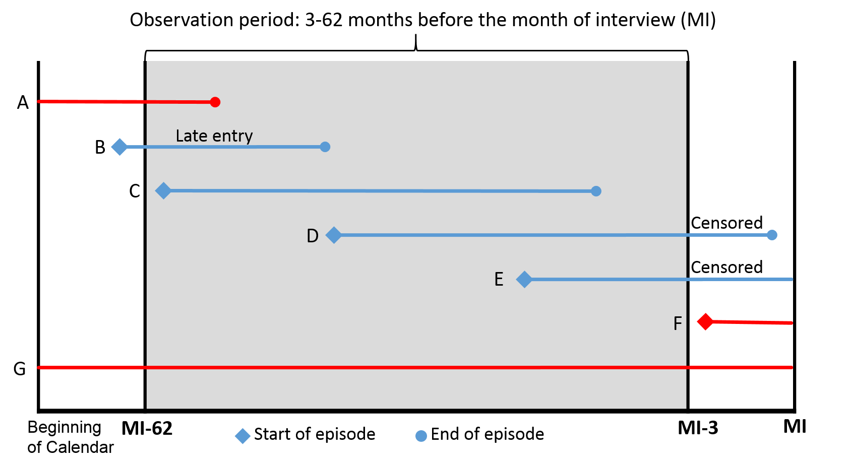
Episodes A and G are excluded as they started before the calendar and we do not have information on the duration of use prior to the calendar. Episode B is included, but as a late entry, as the episode started within the calendar, but outside of the period of interest. Episode C is included as a fully observed episode in the period of interest. Both episodes D and E are included but are censored 3 months before the month of interview. Episode F is excluded as the episode starts outside the period of interest.
E9.0Introductory example
Using the DHS-6 Model Datasets, we first sum each month of exposure in the period of interest (3 to 62 months preceding the survey) according to the duration of use of the method in that month. Late entries will first enter the table at the duration of use when they entered the period of interest. In the month of discontinuation of the method, the discontinuations are tallied according to the reason for discontinuation. The "Any reason" column is the sum of the individual reasons for discontinuation. The "Switched to another method" column is tallied separately from the reasons for discontinuation.
| Duration of use | Method failure | Desire to become pregnant | Other fertility related reasons | Side effects/ health concerns | Wanted more effective method | Other method related reasons | Other reasons | Any reason | Switched to another method | Exposure |
| 1 | 0.887530 | 2.329931 | 0.000000 | 18.885184 | 7.936933 | 1.547109 | 10.400709 | 41.987396 | 3.789610 | 2,631.94 |
| 2 | 1.041063 | 1.140181 | 0.291982 | 9.595957 | 0.737800 | 1.203585 | 0.809309 | 14.819877 | 1.475600 | 2,534.74 |
| 3 | 6.722316 | 9.828108 | 0.399263 | 59.663155 | 8.163438 | 3.252900 | 3.729920 | 91.759100 | 15.687751 | 2,496.58 |
| 4 | 1.584460 | 0.000000 | 1.982117 | 21.353032 | 1.219110 | 7.822816 | 2.456574 | 36.418109 | 5.191382 | 2,331.74 |
| 5 | 5.999001 | 1.686366 | 1.172808 | 4.998823 | 3.576653 | 0.799367 | 0.809309 | 19.042327 | 4.672285 | 2,205.84 |
| 6 | 6.367820 | 19.024693 | 0.000000 | 43.431689 | 6.550592 | 11.890163 | 8.981334 | 96.246291 | 25.541805 | 2,119.36 |
| 7 | 0.903114 | 10.711671 | 0.000000 | 10.925789 | 3.527042 | 0.000000 | 0.394817 | 26.462433 | 5.166854 | 1,954.98 |
| 8 | 3.610944 | 4.739678 | 0.000000 | 9.301247 | 0.000000 | 1.202538 | 16.878426 | 35.732833 | 3.565578 | 1,883.74 |
| 9 | 0.000000 | 14.390345 | 1.092375 | 28.412269 | 8.904068 | 0.257330 | 11.521093 | 64.577480 | 31.959763 | 1,802.60 |
| 10 | 1.315005 | 9.698899 | 1.147836 | 17.394270 | 1.827615 | 0.903114 | 2.339794 | 34.626533 | 9.736157 | 1,697.47 |
| 11 | 4.868782 | 7.380097 | 2.320644 | 5.824226 | 1.827615 | 1.547109 | 3.353669 | 27.122142 | 2.636924 | 1,613.89 |
| 12 | 2.672211 | 15.977691 | 2.616564 | 12.536034 | 6.412058 | 6.683679 | 13.131727 | 60.029964 | 17.138133 | 1,545.51 |
We now convert the counts of discontinuations and the months of exposure into monthly rates of discontinuation (qij) by dividing the discontinuation columns by the exposure column, as below:
| Duration of use | Method failure | Desire to become pregnant | Other fertility related reasons | Side effects/ health concerns | Wanted more effective method | Other method related reasons | Other reasons | Any reason | Switched to another method | 1 | 0.000337 | 0.000885 | 0.000000 | 0.007175 | 0.003016 | 0.000588 | 0.003952 | 0.015953 | 0.001440 | 2 | 0.000411 | 0.000450 | 0.000115 | 0.003786 | 0.000291 | 0.000475 | 0.000319 | 0.005847 | 0.000582 | 3 | 0.002693 | 0.003937 | 0.000160 | 0.023898 | 0.003270 | 0.001303 | 0.001494 | 0.036754 | 0.006284 | 4 | 0.000680 | 0.000000 | 0.000850 | 0.009158 | 0.000523 | 0.003355 | 0.001054 | 0.015618 | 0.002226 | 5 | 0.002720 | 0.000765 | 0.000532 | 0.002266 | 0.001621 | 0.000362 | 0.000367 | 0.008633 | 0.002118 | 6 | 0.003005 | 0.008977 | 0.000000 | 0.020493 | 0.003091 | 0.005610 | 0.004238 | 0.045413 | 0.012052 | 7 | 0.000462 | 0.005479 | 0.000000 | 0.005589 | 0.001804 | 0.000000 | 0.000202 | 0.013536 | 0.002643 | 8 | 0.001917 | 0.002516 | 0.000000 | 0.004938 | 0.000000 | 0.000638 | 0.008960 | 0.018969 | 0.001893 | 9 | 0.000000 | 0.007983 | 0.000606 | 0.015762 | 0.004940 | 0.000143 | 0.006391 | 0.035825 | 0.017730 | 10 | 0.000775 | 0.005714 | 0.000676 | 0.010247 | 0.001077 | 0.000532 | 0.001378 | 0.020399 | 0.005736 | 11 | 0.003017 | 0.004573 | 0.001438 | 0.003609 | 0.001132 | 0.000959 | 0.002078 | 0.016805 | 0.001634 | 12 | 0.001729 | 0.010338 | 0.001693 | 0.008111 | 0.004149 | 0.004325 | 0.008497 | 0.038841 | 0.011089 |
Next we convert the monthly discontinuation rates into the cumulative probabilities of not discontinuing at each month, using the formula li,j = li-1,j - (li-1,any * qij), where l0,j = 1 and l0,any = 1. To carry out these calculations, first calculate l1,any, then l2,any, etc. for "any reason", and then calculate l1,j, l2,j, etc. for each separate reason for discontinuation j.
| Duration of use | Method failure | Desire to become pregnant | Other fertility related reasons | Side effects/ health concerns | Wanted more effective method | Other method related reasons | Other reasons | Any reason (li,any) | Switched to another method | 0 | 1.000000 | 1.000000 | 1.000000 | 1.000000 | 1.000000 | 1.000000 | 1.000000 | 1.000000 | 1.000000 | 1 | 0.999663 | 0.999115 | 1.000000 | 0.992825 | 0.996984 | 0.999412 | 0.996048 | 0.984047 | 0.998560 | 2 | 0.999259 | 0.998672 | 0.999887 | 0.989099 | 0.996698 | 0.998945 | 0.995734 | 0.978294 | 0.997987 | 3 | 0.996624 | 0.994821 | 0.999730 | 0.965720 | 0.993499 | 0.997670 | 0.994273 | 0.942337 | 0.991840 | 4 | 0.995984 | 0.994821 | 0.998929 | 0.957091 | 0.993006 | 0.994509 | 0.993280 | 0.927620 | 0.989742 | 5 | 0.993461 | 0.994112 | 0.998436 | 0.954988 | 0.991502 | 0.994173 | 0.992939 | 0.919612 | 0.987777 | 6 | 0.990698 | 0.985857 | 0.998436 | 0.936143 | 0.988660 | 0.989013 | 0.989042 | 0.877850 | 0.976694 | 7 | 0.990293 | 0.981047 | 0.998436 | 0.931237 | 0.987076 | 0.989013 | 0.988865 | 0.865967 | 0.974374 | 8 | 0.988633 | 0.978868 | 0.998436 | 0.926961 | 0.987076 | 0.988461 | 0.981106 | 0.849541 | 0.972735 | 9 | 0.988633 | 0.972086 | 0.997921 | 0.913571 | 0.982880 | 0.988339 | 0.975676 | 0.819106 | 0.957673 | 10 | 0.987998 | 0.967406 | 0.997367 | 0.905177 | 0.981998 | 0.987903 | 0.974547 | 0.802397 | 0.952975 | 11 | 0.985578 | 0.963737 | 0.996213 | 0.902282 | 0.981089 | 0.987134 | 0.972880 | 0.788913 | 0.951664 | 12 | 0.984214 | 0.955581 | 0.994878 | 0.895883 | 0.977816 | 0.983723 | 0.966177 | 0.758270 | 0.942916 |
Finally, the 12-month discontinuation rates are simply 1 minus the rates of continuing at 12 months:
| Duration of use | Method failure | Desire to become pregnant | Other fertility related reasons | Side effects/ health concerns | Wanted more effective method | Other method related reasons | Other reasons | Any reason (li,any) | Switched to another method |
| 12 | 0.015786 | 0.044419 | 0.005122 | 0.104117 | 0.022184 | 0.016277 | 0.033823 | 0.241730 | 0.057084 |
Or, as percentages:
| 12 | 1.6 | 4.4 | 0.5 | 10.4 | 2.2 | 1.6 | 3.4 | 24.2 | 5.7 |
Next section: Example 9 - Twelve-month discontinuation, failure, and switching rates
Module 6: Contraceptive discontinuation, failure and switching rates
Goal of the module: For analysts to understand how contraceptive discontinuation rates and switching rates are calculated, and how to use the event files to produce the rates. Though this model has detailed example and offers code on Stata and SPSS, it is recommended to first review the Guide to DHS Statistics to understand how contraceptive discontinuation rates are calculated.
6.2 How to calculate discontinuation rates
Though discontinuation rates make use of straightforward demographic methods to calculate cumulative discontinuations, we must manipulate the data differently depending on whether Stata or SPSS is used for analysis. With both software programs, we will roughly follow the same six steps for constructing the discontinuation rate table:
- 1) Calculate exposure, late entries, and censoring for the period 3-62 months prior to interview
- 2) Recode methods, reasons for discontinuation, and create switching variable
- 3) Calculate competing risks cumulative incidence
- 4) Calculate weighted and unweighted denominators
- 5) Combine components for table output
- 6) Output table
Example 9 - Twelve-month discontinuation, failure, and switching rates
Logic for example 9 can be found in the following files:
| Software | Commands | Output |
|---|---|---|
| Stata | Stata\Example9.do | Stata\Example9.log |
| SPSS | SPSS\Example9.sps | SPSS\Example9.txt |
E9.1Calculate exposure, late entries and censoring for the period 3-62 months prior to interview
If using Stata, first install stcompet if not already installed before starting at Step 1.
Once we open the events file created in Module 5, we need leave out episodes that do not contribute exposure time to this multiple decrement life table.
Begin by dropping episodes that were ongoing when the calendar began (v017=ev900), and drop births, terminations, and pregnancies. We calculate the time of the beginning of the episode (tbeg_int = v008 – ev900) and the end of the episode (tend_int = v008 – ev901), and generate variables for discontinuations and for late entries. By using the variables for the months an episode began (tbeg_int) and ended (tend_int), we can censor the calendar to five years of data and still include late entries (v008-ev901>62), to calculate the exposure within the window of 3-62 months prior to the interview.
Some analysts prefer to exclude female sterilization when calculating all method discontinuation rates, and others prefer to exclude all late entries. The DHS Program does not exclude either of these cases in the discontinuation rates produced.
* DHS Calendar Tutorial - Example 9
* Calculating discontinuation rates using event files

* note that the denominator in this table is all women, including sterilized women
* also includes missing methods to match the final reports

* if you don't have stcompet installed, use the line below to find it and follow instructions to install it:
//findit stcompet

* change to a working directory where the data are stored
* or add the full path to the 'use' command below
cd "C:\Data\DHS_model"

* open the event file dataset created by the 'create events file.do'
use "eventsfile.dta", clear


* Step 1
* calculate exposure, late entries and censoring for the period 3-62 months prior to the interview

*gen wt
gen wt = v005/1000000

* drop events that were ongoing when calendar began
drop if v017 == ev900

* drop births, terminations, pregnancies, and episodes of non-use
* keep missing methods. to exclude missing change 99 below to 100.
drop if (ev902 > 80 & ev902 < 99) | ev902==0

* time from beginning of event to interview
gen tbeg_int = v008 - ev900
label var tbeg_int "time from beginning of event to interview"

* time from end of event to interview
gen tend_int = v008 - ev901
label var tend_int "time from end of event to interview"

* discontinuation variable
gen discont = 0
replace discont = 1 if ev903 != 0

* censoring those who discontinue in last three months
replace discont = 0 if tend_int < 3
label var discont "discontinuation indicator"
tab discont
tab ev903 discont, m

* generate late entry variable
gen entry = 0
replace entry = tbeg_int - 62 if tbeg_int >= 63
tab tbeg_int entry

* taking away exposure time outside of the 3 to 62 month window
gen exposure = ev901a
replace exposure = ev901a - (3 - tend_int) if tend_int < 3
recode exposure -3/0=0

* drop those events that started in the month of the interview and two months prior
drop if tbeg_int < 3

* drop events that started and ended before 62 months prior to survey
drop if tbeg_int > 62 & tend_int > 62

* to remove sterilized women from denominator use the command below - not used for DHS standard
//replace exposure = . if ev902 == 6

* censor any discontinuations that are associated with use > 59 months
* not censored in this example
//replace discont = 0 if (exposure - entry) > 59
* DHS Calendar Tutorial - Example 9.
* Calculating discontinuation rates using event files.

* note that the denominator in this table is all women, and includes sterilized women
* and also includes missing methods to match the final reports.

* change to a working directory where the data are stored
* or add the full path to the 'use' command below.
cd "C:\Data\DHS_model".

* open the event file dataset created by the 'create events file.sps'.
get file="eventsfile.sav".
* name the dataset.
dataset name eventsfile.


* Step 1.
* calculate exposure, late entries and censoring for the period 3-62 months prior to the interview.

* weight variable.
compute wt=v005/1000000.
* weight will be applied later when we need it in step 3.

* drop events that were ongoing when calendar began,
* keeping those that started after the start of the calendar.
select if (ev900 > v017).

* drop births, terminations, pregnancies, and episodes of non-use
* keep missing methods. to exclude, drop "| ev902 = 99".
select if (ev902 <> 0 & (ev902 < 80 | ev902 = 99)).

* time from beginning of event to interview.
compute tbeg_int = v008 - ev900.
variable labels tbeg_int "time from beginning of event to interview".

* time from end of event to interview.
compute tend_int = v008 - ev901.
variable labels tend_int "time from end of event to interview".
formats tbeg_int tend_int (f2.0).

* discontinuation variable.
compute discont = 0.
if (ev903 <> 0) discont = 1.

* censoring those who discontinue in last three months.
if (tend_int < 3) discont = 0.
variable labels discont "Discontinuation indicator".
value labels discont 0 "No discontinuation" 1 "Discontinuation".
formats discont (f1.0).
frequencies variables=discont.
crosstabs tables=ev903 by discont /cells=count column /count=asis.

* generate late entry variable.
compute entry = 0.
if (tbeg_int >= 63) entry = tbeg_int - 62.
variable labels entry "Late entry months".
formats entry (f1.0).
crosstabs tables=tbeg_int by entry /count=asis.

* taking away exposure time outside of the 3 to 62 month window.
compute exposure = ev901a.
if (tend_int < 3) exposure = ev901a - (3 - tend_int).
recode exposure (-3 thru 0=0).
variable labels exposure "Exposure".
formats exposure (f2.0).

* drop those events that started in the month of the interview and two months prior.
select if (tbeg_int >= 3).
* drop events that started and ended before 62 months prior to survey.
select if (tbeg_int <= 62 | tend_int <= 62).

* to remove episodes from sterilized women from denominator use the command below - not for DHS standard.
/* if (ev902 = 6) exposure=$sysmis. */

* censor any discontinuations that are associated with use > 59 months.
* not censored in this example.
/* if ((exposure - entry) > 59) discont = 0. */
E9.2Recode methods, reasons for discontinuations, and create switching variable
After the exposure time has been calculated, we now need to recode the methods (ev902) and reasons for discontinuation (ev903) of interest before doing any analysis. Because there are many methods, it is advised to group where possible – in the example below, several less common methods are grouped into an "Other" category. In many surveys there is interest in calculating discontinuation rates for IUD, Periodic Abstinence, and Withdrawal, but in the Model dataset these are too few cases, so these are also grouped into the "Other" category. When recoding discontinuations, it should be noted that when analyzing competing risks in Stata, only seven competing risks can be handled in the analysis at a time. Although this can be overcome by reorganizing discontinuations and running the analysis more than once, in this example, we conveniently want to recode our reasons for discontinuation into seven major categories.
To create a switching variable, we will look for places where the end of an event is one month less than the start of a new event (ev901=ev900[_n+1]). We must also account for women who discontinued a method because they wanted a more effective method (ev903=7) and switched to a new method with no more than a one-month gap (ev901=ev900[_n+2] & ev905=0).
* Step 2
* recode methods, discontinuation reason, and construct switching
* recode contraceptive method
* IUD, Periodic Abstinence, and Withdrawal skipped and grouped with other due to small numbers of cases
recode ev902                          ///
    (1  = 1 "Pill")                   ///
/*  (2  = 2 "IUD") */                 ///
    (3  = 3 "Injectables")            ///
    (11 = 4 "Implant")                ///
    (5  = 5 "Male condom")            ///
/*  (8  = 6 "Periodic abstinence") */ ///
/*  (9  = 7 "Withdrawal") */          ///
    (13 18 = 8 "LAM/EC")              ///
    (nonmissing = 9 "Other")          ///
    (missing = .), gen(method)
tab ev902 method, m
* LAM and Emergency contraception are grouped here
* Other category is Female Sterilization, Male sterilization, Other Traditional,
*       Female Condom, Other Modern, Standard Days Method
* plus IUD, Periodic Abstinence, Withdrawal
* adjust global meth_list below if changing the grouping of methods above

* change name of reasons label list to avoid labels we don't want
label copy reason ev903
label val ev903 ev903
label drop reason // we don't want the labels for reason being copied to var reason

* recode reasons for discontinuation - ignoring switching
recode ev903                                         ///
    (0 .     = .)                                    ///
    (1       = 1 "Method failure")                   ///
    (2       = 2 "Desire to become pregnant")        ///
    (9 12 13 = 3 "Other fertility related reasons")  ///
    (4 5     = 4 "Side effects/health concerns")     ///
    (7       = 5 "Wanted more effective method")     ///
    (6 8 10  = 6 "Other method related")             ///
    (nonmissing = 7 "Other/DK") if discont==1, gen(reason)
label var reason "Reason for discontinuation"
tab reason
tab ev903 reason if discont==1, m

* switching methods
* switching directly from one method to the next, with no gap
sort caseid ev004
by caseid: gen switch = 1 if ev901+1 == ev900[_n+1]
* if reason was "wanted more effective method" allow for a 1-month gap
by caseid: replace switch = 1 if ev903 == 7 & ev901+2 >= ev900[_n+1] & ev905 == 0
* not a switch if returned back to the same method
* note that these are likely rare, so there may be no or few changes from this command
by caseid: replace switch = . if ev902 == ev902[_n+1] & ev901+1 == ev900[_n+1]
tab switch

* calculate variable for switching for discontinuations we are using
gen discont_sw = .
replace discont_sw = 1 if switch == 1 & discont == 1
replace discont_sw = 2 if discont_sw == . & ev903 != 0 & ev903 != . & discont == 1
label def discont_sw 1 "switch" 2 "other reason"
label val discont_sw discont_sw
tab discont_sw
* Step 2.
* Recode methods, reasons for discontinuations, and create switching variable.

* recode contraceptive method.
* IUD, Periodic Abstinence, and Withdrawal skipped and grouped with other due to small numbers of cases.
recode ev902
  (sysmis = sysmis)
  (1 = 1) /*(2 = 2)*/ (3 = 3) (11 = 4) (5 = 5) /*(8 = 6)*/ /*(9 = 7)*/ (13 18 = 8) (else = 9)
  into method.
variable labels method "Contraceptive method".
value labels method
  1 "Pill"
  2 "IUD"
  3 "Injectables"
  4 "Implant"
  5 "Male condom"
  6 "Periodic abstinence"
  7 "Withdrawal"
  8 "LAM/EC"
  9 "Other [6]"
 99 "All methods". /* used later */
* LAM and Emergency contraception are grouped here.
* Other category is Female Sterilization, Male sterilization, Other Traditional,
*   Female Condom, Other Modern, Standard Days Method.
*   plus IUD, Periodic Abstinence, Withdrawal.

formats method (f1.0).
crosstabs tables=ev902 by method /count=asis.

* filter for discontinuations only.
compute filter$ = (discont = 1).
filter by filter$.
* recode reasons for discontinuation - ignoring switching.
recode ev903
  (0 sysmis = sysmis)
  (1       = 1 /* Method failure */)
  (2       = 2 /* Desire to become pregnant */)
  (9 12 13 = 3 /* Other fertility related reasons */)
  (4 5     = 4 /* Side effects/health concerns */)
  (7       = 5 /* Wanted more effective method */)
  (6 8 10  = 6 /* Other method related */)
  (else    = 7 /* Other/DK */)
  into reason.
variable labels reason "Reason for discontinuation".
value labels reason
  1 "Method failure"
  2 "Desire to become pregnant"
  3 "Other fertility related reasons"
  4 "Side effects/health concerns"
  5 "Wanted more effective method"
  6 "Other method related"
  7 "Other/DK".
formats reason (f1.0).
if (discont <> 1) reason = $sysmis.
frequencies variables=reason.
crosstabs tables=ev903 by reason /count=asis.
filter off.

* switching methods.
* switching directly from one method to the next, with no gap.
sort cases by caseid ev004 (d).
if (caseid = lag(caseid) & ev901+1 = lag(ev900)) switch = 1.
* if reason was "wanted more effective method" allow for a 1-month gap.
if (ev903 = 7 & ev905 = 0 & caseid = lag(caseid) & ev901+2 >= lag(ev900)) switch = 1.

* not a switch if returned back to the same method.
* there should be none of these, so there should be no changes from this command.
if (caseid = lag(caseid) & ev902 = lag(ev902) & ev901+1 = lag(ev900)) switch = $sysmis.

variable labels switch "Switching method".
value labels switch 1 "Switched method".
formats switch (f1.0).
frequencies variables=switch.

* calculate variable for switching for discontinuations we are using.
compute discont_sw=$sysmis.
if (switch = 1 & discont = 1) discont_sw = 1.
if (sysmis(discont_sw) & ev903 <> 0 & not sysmis(ev903) & discont = 1) discont_sw = 0.
variable labels discont_sw "Discontinuation for switching".
value labels discont_sw 1 "Switch" 0 "Other reason".
formats discont_sw (f1.0).
frequencies variables=discont_sw.
E9.3Calculate the competing risks cumulative incidence for each method and for total
Using the variables created in E9.1 and E9.2, we can calculate cumulative incidence of discontinuations for each method and for all methods, regarding the reasons for discontinuation as competing risks.
In Stata we first declare the data to be survival-time data using stset. The time variable will be our exposure variable, and we will use our entry to indicate when the record comes under observation and use our reason variable as a failure event. Now we can use the stcompet command, which generates variables containing cumulative incidence for each of the competing risks. We must list the competing risks as values that compete with the failure event variable from the stset in the line of code above. We will save the resulting dataset, which will have the discontinuation rate for each method attached to each case.
* Step 3
* Calculate the competing risks cumulative incidence for each method and for all methods

* create global lists of the method variables included
levelsof method
global meth_codes `r(levels)'
*modify meth_list and methods_list according to the methods included
*global meth_list pill IUD inj impl mcondom pabst withdr lamec other
*global methods_list `" "Pill" "IUD" "Injectables" "Implant" "Male condom" "Periodic abstinence" "Withdrawal" "LAM/EC" "Other" "All methods" "'
global meth_list pill inj impl mcondom pabst other
global methods_list `" "Pill" "Injectables" "Implant" "Male condom" "LAM/EC" "Other" "All methods" "'
global drate_list
global drate_list_sw
foreach m in $meth_list {
    global drate_list $drate_list drate_`m'
    global drate_list_sw $drate_list_sw drate_`m'_sw
}

* competing risks estimates - first all methods and then by method
tokenize allmeth $meth_list
foreach x in 0 $meth_codes {

    * by reason - no switching
    * declare time series data for st commands
    stset exposure if `x' == 0 | method == `x' [iw=wt], failure(reason==1) enter(entry)
    stcompet discont_`1' = ci, ///
        compet1(2) compet2(3) compet3(4) compet4(5) compet5(6) compet6(7)
    * convert rate to percentage
    gen drate_`1' = discont_`1' * 100

    * switching
    * declare time series data for st commands
    stset exposure if `x' == 0 | method == `x' [iw=wt], failure(discont_sw==1) enter(entry)
    stcompet discont_`1'_sw = ci, compet1(2)
    * convert rate to percentage
    gen drate_`1'_sw = discont_`1'_sw * 100

    * Get the label for the method and label the variables appropriately
    local lab1 All methods
    if `x' > 0 {
        local lab1 : label method `x'
    }
    label var drate_`1' "Rate for `lab1'"
    label var drate_`1'_sw "Rate for `lab1' for switching"

    * shift to next method name in token list
    macro shift
}

* keep just the variables we need for output
keep caseid method drate* exposure reason discont_sw wt entry

* save data file with cumulative incidence variables added to each case
save "drates.dta", replace
* Step 3.
* Calculate the competing risks cumulative incidence for each method and for total.
weight by wt.

* Split reason for discontinuation into separate 0/1 variables.
recode reason (1 = 1)(else = 0) into reason_1.
recode reason (2 = 1)(else = 0) into reason_2.
recode reason (3 = 1)(else = 0) into reason_3.
recode reason (4 = 1)(else = 0) into reason_4.
recode reason (5 = 1)(else = 0) into reason_5.
recode reason (6 = 1)(else = 0) into reason_6.
recode reason (7 = 1)(else = 0) into reason_7.
variable labels
  reason_1 "Method failure"
  reason_2 "Desire to become pregnant"
  reason_3 "Other fertility related reasons"
  reason_4 "Side effects/health concerns"
  reason_5 "Wanted more effective method"
  reason_6 "Other method related"
  reason_7 "Other/DK".
formats reason_1 reason_2 reason_3 reason_4 reason_5 reason_6 reason_7 (f1.0).

* Aggregate counts by exposure of totals exposure (N) and discontinuations for each reason.
* by method.
dataset declare aggr_meth.
aggregate
  /outfile='aggr_meth'
  /break=method exposure
  /discont =sum(discont)
  /reason_1=sum(reason_1)
  /reason_2=sum(reason_2)
  /reason_3=sum(reason_3)
  /reason_4=sum(reason_4)
  /reason_5=sum(reason_5)
  /reason_6=sum(reason_6)
  /reason_7=sum(reason_7)
  /discont_sw=sum(discont_sw)
  /expo=N
  /expo_u=NU.

* for All methods.
dataset declare aggr_all.
aggregate
  /outfile='aggr_all'
  /break=exposure
  /discont =sum(discont)
  /reason_1=sum(reason_1)
  /reason_2=sum(reason_2)
  /reason_3=sum(reason_3)
  /reason_4=sum(reason_4)
  /reason_5=sum(reason_5)
  /reason_6=sum(reason_6)
  /reason_7=sum(reason_7)
  /discont_sw=sum(discont_sw)
  /expo=N
  /expo_u=NU.

* combine file of exposure for all methods and by method into one.
dataset activate aggr_meth.
add files
  /file=*
  /file='aggr_all'.
execute.

* recode missing to 99 for all methods.
recode method (sysmis = 99).

* Switch back to the events file for the late entries.
dataset activate eventsfile.

* Aggregate counts of late entries - to be removed later from cumulative exposure.
* by method.
dataset declare aggr_late_meth.
aggregate
  /outfile='aggr_late_meth'
  /break=method entry
  /lateentry=N
  /lateentry_u=NU.

* for All methods.
dataset declare aggr_late_all.
aggregate
  /outfile='aggr_late_all'
  /break=entry
  /lateentry=N
  /lateentry_u=NU.

* combine file of late entries for all methods and by method into one.
dataset activate aggr_late_meth.
add files
  /file=*
  /file='aggr_late_all'.
execute.

* recode missing to 99 for all methods.
recode method (sysmis = 99).

* drop cases without late entry (entry = 0).
select if (entry >  0).
* rename late entry variable to exposure.
rename variables entry = exposure.

* merge the exposure and late entries files into one file by method and exposure.
dataset activate aggr_meth.
match files
  /file = *
  /table = 'aggr_late_meth'
  /by method exposure.

* set any missing late entries and any missing switching to 0.
if (sysmis(lateentry)) lateentry = 0.
if (sysmis(lateentry_u)) lateentry_u = 0.
if (sysmis(discont_sw)) discont_sw = 0.
execute.

* close separate files that are no longer needed.
dataset close aggr_all.
dataset close aggr_late_all.
dataset close aggr_late_meth.
dataset close eventsfile.


* Accumulate the exposure and the episodes for the prior months.

* reverse the order of the file so longest exposure first to allow for cumulation of the exposures.
sort cases method (a) exposure (d).
* initialize the cumulative exposure to 0.
compute cum_expo = 0.
compute episodes = 0.
compute cum_expo_u = 0.
* if the last month (first entry) for the method, set the cumulative exposure to the monthly exposure minus the late entries.
if (missing(lag(method)) or method<>lag(method)) cum_expo = expo - lateentry.
if (missing(lag(method)) or method<>lag(method)) episodes = expo.
if (missing(lag(method)) or method<>lag(method)) cum_expo_u = expo_u - lateentry_u.
* if not the last month (first entry) for the method,
* set the cumulative exposure to the previous months cumulative exposure plus the monthly exposure minus the late entries.
if (method=lag(method)) cum_expo = lag(cum_expo) + expo - lateentry.
if (method=lag(method)) episodes = lag(episodes) + expo.
if (method=lag(method)) cum_expo_u = lag(cum_expo_u) + expo_u - lateentry_u.
execute.

* drop the cases beyond 12 months exposure now as we are only interested in 12 month discontinuation rates.
* change to 24 or 36 if two year or three year discontinuation rates are desired.
select if (exposure <= 12).
* resort the data to enable the calculation of the life table.
sort cases method (a) exposure (a).


* Monthly rates of discontinuation.
* Convert counts of discontinuation and switching rates to monthly rates.
compute discont = discont/cum_expo.
compute discont_sw = discont_sw/cum_expo.
compute reason_1 = reason_1/cum_expo.
compute reason_2 = reason_2/cum_expo.
compute reason_3 = reason_3/cum_expo.
compute reason_4 = reason_4/cum_expo.
compute reason_5 = reason_5/cum_expo.
compute reason_6 = reason_6/cum_expo.
compute reason_7 = reason_7/cum_expo.

* Construct the life table.
do if (exposure = 1).
* First month of life table = 1 minus the monthly rate for month 1.
+ compute lt_reason_1 = 1 - reason_1.
+ compute lt_reason_2 = 1 - reason_2.
+ compute lt_reason_3 = 1 - reason_3.
+ compute lt_reason_4 = 1 - reason_4.
+ compute lt_reason_5 = 1 - reason_5.
+ compute lt_reason_6 = 1 - reason_6.
+ compute lt_reason_7 = 1 - reason_7.
+ compute lt_discont = 1 - discont.
+ compute lt_discont_sw = 1 - discont_sw.
else.
* remaining months.
+ compute lt_reason_1 = lag(lt_reason_1) - (lag(lt_discont) * reason_1).
+ compute lt_reason_2 = lag(lt_reason_2) - (lag(lt_discont) * reason_2).
+ compute lt_reason_3 = lag(lt_reason_3) - (lag(lt_discont) * reason_3).
+ compute lt_reason_4 = lag(lt_reason_4) - (lag(lt_discont) * reason_4).
+ compute lt_reason_5 = lag(lt_reason_5) - (lag(lt_discont) * reason_5).
+ compute lt_reason_6 = lag(lt_reason_6) - (lag(lt_discont) * reason_6).
+ compute lt_reason_7 = lag(lt_reason_7) - (lag(lt_discont) * reason_7).
+ compute lt_discont = lag(lt_discont) - (lag(lt_discont) * discont).
+ compute lt_discont_sw = lag(lt_discont_sw) - (lag(lt_discont) * discont_sw).
end if.
execute.
formats lt_reason_1 lt_reason_2 lt_reason_3 lt_reason_4 lt_reason_5 lt_reason_6 lt_reason_7 lt_discont lt_discont_sw (f8.6).
In SPSS the standard life table procedures do not produce results that match the results that DHS presents, so it is necessary to calculate the life table in a more manual process, following the procedure described in section 6.1. The main difference is that the life table procedures such as survival count only half a month of exposure in the month of discontinuation, whereas the DHS approach uses a full month of exposure in the month of discontinuation.
We first create dichotomous variables for each reason for discontinuation category, and then aggregate the episode data by exposure for all reasons for discontinuation combined, each separate reason, and for switching. We do this first for all methods and then by each method group. Similarly, we aggregate the late entries for all methods and for each method group. We append these files together, and recode any missing values for late entries or switching to 0, and we recode the missing value for all methods to code 99. This gives a file of discontinuations and switching by method and total exposure.
We next sort the data in descending order by exposure within method and accumulate the exposure into the prior months to calculate the full exposure starting from the first month of use, subtracting out the late entries. We also accumulate the total episodes in the same way, but including the late entries. At this point, we can drop all exposure beyond 12 months as we are only interested in the 12-month discontinuation rates. The result is the data in the first table under E9.0, for all methods and also by method.
Now we convert the counts of discontinuations and exposure into monthly rates of discontinuation by dividing the reasons for discontinuation and switching by the exposure, as found in the second table under E9.0. Next, these are converted into a life table table of cumulative probabilities of not discontinuing or switching.
At the end of this step we have a dataset of probabilities of not discontinuing or switching with methods in the rows and reasons for discontinuation or switching in the columns - the opposite of the Stata version above, which has methods in the columns.
E9.4Calculate weighted and unweighted denominators
Once the discontinuation rates for each method and all methods combined are saved, we will move on to calculating weighted and unweighted denominators. The unweighted denominator is a count of episodes in the first month and can be used to determine if a cell has enough power to be reported. With discontinuation rates, The DHS Program does not show rates for methods that have less than 125 months of exposure in the first month of the life due to large sampling variance. Methods that have 125-249 months of exposure are shown in parentheses to caution the reader that estimates of the discontinuation rates are based on small sample sizes.
In Stata, we drop late entries, and then a simple count by method can be used to calculate the unweighted episodes per method in the first month of exposure. Save this dataset, we will merge this to the weighted denominators once we calculate them.
For weighted denominators, use the dataset saved at the end of E9.3, and count all episodes again (this time including late entries) being sure to weight them this time. Then merge back in the unweighted denominators using the variable method to link the denominators by method.
At this point we have two columns of denominators (see below), and we must transpose the rows and columns using xpose so the weighted and unweighted Ns become rows that will later be appended to the discontinuation rates.
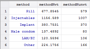
After transposing and renaming the columns to match the methods they represent (see below), save the dataset.
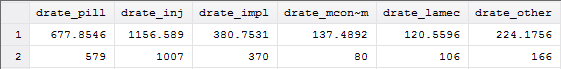
* Step 4
* calculate and save the weighted and unweighted denominators
* and convert into format for adding to dataset of results

* calculate unweighted Ns, for entries in the first month of the life table
drop if entry != 0
collapse (count) methodNunwt = entry, by(method)
save "method_Ns.dta", replace

use "drates.dta", clear
* calculate weighted Ns, for total episodes including late entries
collapse (count) methodNwt = entry [iw=wt], by(method)

* merge in the unweighted Ns
merge 1:1 method using "method_Ns.dta"

* drop the merge variable
drop _merge

* switch rows (methods) and columns (weighted and unweighted counts)
* to create a file that will have a row for weight Ns and a row for unweighted Ns with methods as the variables
* first transpose the file
xpose, clear
* rename the variables v1 to v9 to match the drate variable list (ignoring all methods)
tokenize $drate_list
local num : list sizeof global(drate_list)
forvalues x = 1/`num' { // this list is a sequential list of numbers up to the count of vars
    rename v`x' `1'
    mac shift
}
* drop the first line with the method code as the methods are now variables
drop if _n == 1
* generate the reason code (to be used last for the Ns)
gen reason = 9 + _n

* save the final Ns - two rows, one for weighhted N, one for unweighted N
save "method_Ns.dta", replace
* Step 4.
* Total episodes, including late entries can be found in first row of life table
  use offset of 11 from 12th row to point to first.
if (exposure = 12) nepisodes = lag(episodes,11).
if (exposure = 12) nexpo_u = lag(cum_expo_u,11).
variable labels
  nepisodes "Number of episodes of use [5]"
 /nexpo_u "Unweighted exposure in first month".
formats nepisodes nexpo_u (f6.0).
execute.
In SPSS, the handling of the exposure and unweighted denominator is carried out in the prior step (Step 3), as we accumulated the table to produce the life table, and all that is needed here is to extract the weighted number of episodes and the unweighted exposure from the first month for each method.
E9.5Combine components for output table
At this point, the rates have been calculated, but in Stata they are attached to each episode use from the original file, saved in drates.dta, while in SPSS we already have an aggregated file of discontinuation rates.
In Stata we now must collapse the data by reason for discontinuation, all reasons combined, and switching. Once we append these all together, we will have a final table of discontinuation rates.
In SPSS, we just need to select the rows for exposure at 12 months and then calculate the 12-month discontinuation rates as 1 minus the cumulative probability of not discontinuing at 12 months of exposure for each reason, all reasons, and for switching.
* Step 5
* Prepare resulting data for output
* This code can be used to produce rates for different durations for use,
* but is here set for 12-month discontinuation rates

* Loop through possible discontinuation rates for 6, 12, 24 and 36 months
//foreach x in 6 12 24 36 {
* current version presents only 12-month discontinuation rates:
local x 12

* open the working file with the rates attached to each case
use "drates.dta", clear

* collect information from relevant time period only
drop if exposure > `x'

* keep only discontinuation information
keep method drate* exposure reason discont_sw wt

* save smaller dataset for x-month duration which we will use in collapse commands below
save "drates_`x'm.dta", replace

* collapsing data for reasons, all reasons, switching, merging and adding method Ns
* reasons for discontinuation
* collapse data by discontinuation category and save
collapse (max) $drate_list drate_total, by(reason)
* drop missing values
drop if reason == .
save "reasons.dta", replace

* All reasons
* calculate total discontinuation and save
collapse (sum) $drate_list drate_total
gen reason = 8
save "allreasons.dta", replace

* switching data
use "drates_`x'm.dta"
* collapse and save a file just for switching
collapse (max) $drate_list_sw drate_total_sw, by(discont_sw)
* only keep row for switching, not for other reasons
drop if discont_sw != 1
* we no longer need discont_sw and don't want it in the resulting file
drop discont_sw
gen reason = 9  // switching
* rename switching variables to match the non-switching names
rename drate_*_sw drate_*
save "switching.dta", replace

* Go back to data by reasons and merge "all reasons" and switching data to it
use "reasons.dta"
append using "allreasons.dta" // all reasons
append using "switching.dta" // switching
append using "method_Ns.dta" // weighted and unweighted numbers
label def reason 8 "All reasons" 9 "Switching" 10 "Weighted N" 11 "Unweighted N", add

* replace empty cells with zeros for each method
* and sum the weighted and unweighted Ns into the method total variable
foreach z in drate_total $drate_list {
    replace `z' = 0 if `z' == .
    * sum the method Ns to give the total Ns
    replace drate_total = drate_total + `z' if reason >= 10
}
save "drates_`x'm.dta", replace
* Step 5.
* Select just the 12 months exposure to report.
select if (exposure = 12).
* Now extract 12 month discontinuation rates.
+ compute disc_reason_1 = 100* (1 - lt_reason_1).
+ compute disc_reason_2 = 100* (1 - lt_reason_2).
+ compute disc_reason_3 = 100* (1 - lt_reason_3).
+ compute disc_reason_4 = 100* (1 - lt_reason_4).
+ compute disc_reason_5 = 100* (1 - lt_reason_5).
+ compute disc_reason_6 = 100* (1 - lt_reason_6).
+ compute disc_reason_7 = 100* (1 - lt_reason_7).
+ compute disc_any      = 100* (1 - lt_discont).
+ compute disc_switch   = 100* (1 - lt_discont_sw).
formats disc_reason_1 disc_reason_2 disc_reason_3 disc_reason_4 disc_reason_5
        disc_reason_6 disc_reason_7 disc_any disc_switch (f5.1).
variable labels
  disc_reason_1 "Method failure"
  disc_reason_2 "Desire to become pregnant"
  disc_reason_3 "Other fertility related reasons [1]"
  disc_reason_4 "Side effects/health reasons"
  disc_reason_5 "Wanted more effective method"
  disc_reason_6 "Other method related reasons [2]"
  disc_reason_7 "Other/DK"
  disc_any "Any reason [3]"
  disc_switch "Switched to another method [4]".
Both the Stata and the SPSS methods result in a dataset of discontinuation rates, but oriented in opposite directions due to the approaches used to produce them. It can be seen though that the results are the same.
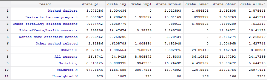
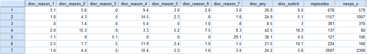
E9.6Output results
Now that we have calculated discontinuation rates, merged in unweighted and weighted denominators, and saved a dataset with all of our components, we can output our results.
In Stata, we have several options for outputting the results, including list, outsheet, or we can use putexcel to directly place each value from our results table into specific Excel cells.
Another option in Stata is to reshape the data for use with other tabulation commands using the reshape long command in Stata. This will change data from a wide format (Stata output above) with reasons for discontinuation in rows and discontinuation rates for each method as columns to a long data set where there are multiple records for each reason for discontinuation to accommodate every reason and method combination. This allows for an easier tabulation in Stata (table method reason [iw=drate_]).
In SPSS, a ctable can be used to tabulate method by the various reasons for discontinuation.
* Step 6
* Output results in various ways

* simple output with reasons in rows and methods in columns
list reason $drate_list drate_allmeth, tab div abb(16) sep(9) noobs linesize(160)
outsheet reason $drate_list drate_allmeth using `x'm_rates.csv, comma replace

* Outputting as excel file with putexcel
* putexcel output
putexcel set "drates_`x'm.xlsx", replace
putexcel B1 = "Reasons for discontinuation"
putexcel A2 = "Contraceptive method"
* list out the contraceptive methods
local row = 2
foreach method of global methods_list {
    local row = `row'+1
    putexcel A`row' = "`method'"
}

putexcel B3:J`row', nformat(number_d2)
putexcel K3:L`row', nformat(number)

tokenize B C D E F G H I J K L
local recs = [_N]
* loop over reasons for discontinuation
forvalues j = 1/`recs' {
    local lab1 : label reason `j'
    putexcel `1'2 = "`lab1'", txtwrap
    local k = 2
    * loop over contraceptive methods
    local str
    foreach i in $drate_list drate_allmeth {
        local k = `k'+1
        local str `str' `1'`k' = `i'[`j']
    }
    * output results for method
    putexcel `str'
    mac shift
}

* Converting results dataset into long format for use with other tab commands

* convert results into long format
reshape long drate_, i(reason) j(method_name) string
gen method = .
tokenize $meth_list allmeth
foreach m in $meth_codes 10 {
    replace method = `m' if method_name == "`1'"
    mac shift
}
label var method "Contraceptive method"
label def method          ///
 1 "Pill"                 ///
 2 "IUD"                  ///
 3 "Injectables"          ///
 4 "Implant"              ///
 5 "Male condom"          ///
 6 "Periodic abstinence"  ///
 7 "Withdrawal"           ///
 8 "LAM/EC"               ///
 9 "Other"                ///
10 "All methods"
label val method method

* Now tabulate (using table instead of tab to avoid extra Totals)
table method reason [iw=drate_], cellwidth(10) f(%3.1f)


* close loop if multiple durations used and file clean up
* closing brace if foreach is used for different durations
//}


* clean up working files
erase "drates.dta"
erase "reasons.dta"
erase "allreasons.dta"
erase "switching.dta"
erase "method_Ns.dta"
* Step 6.
* Output the table.
ctables
  /vlabels variables=method display=none
  /vlabels variables=disc_reason_1 disc_reason_2 disc_reason_3 disc_reason_4 disc_reason_5
                     disc_reason_6 disc_reason_7 disc_any disc_switch nepisodes nexpo_u display=label
  /format maxcolwidth=55
  /table method [c] by
  (disc_reason_1 + disc_reason_2 + disc_reason_3 + disc_reason_4 +
   disc_reason_5 + disc_reason_6 + disc_reason_7 + disc_any + disc_switch) [s] [mean,'',f6.1] + (nepisodes + nexpo_u) [s] [mean,'',f8.0]
  /categories var=all empty=exclude missing=exclude
  /slabels visible=no
  /titles title=
  "Table 7.11 Twelve-month contraceptive discontinuation rates"
  "Among episodes of contraceptive use experienced within the 5 years preceding the survey, "+
  "percentage of episodes discontinued within 12 months, according to reason for "+
  "discontinuation and specific method, DHS-6 Model Data"
  corner="Contraceptive method"
  caption=
  "Note: Figures are based on life table calculations using information on episodes of "+
  "use that occurred 3-62 months preceding the survey"
  "[1] Includes infrequent sex/husband away, difficult to get pregnant/menopausal, "+
  "and marital dissolution/separation"
  "[2] Includes lack of access/too far, costs too much, and inconvenient to use"
  "[3] Reasons for discontinuation are mutually exclusive and add to the total given in "+
  "this column"
  "[4] A woman is considered to have switched to another method if she used a different method "+
  "in the month following discontinuation or if she gave 'wanted a more effective method' "+
  "as the reason for discontinuation and started another method within two months "+
  "of discontinuation."
  "[5] All episodes of use that occur within the 5 years preceding the survey are included. "+
  "Episodes of use include episodes that were discontinued during the period of observation "+
  "and episodes of use that were not discontinued during the period of observation."
  "[6] Includes Female Sterilization, Male sterilization, Other Traditional, Female Condom, "+
  "Other Modern, Standard Days Method plus IUD, Periodic Abstinence, and Withdrawal.".
The resulting output is the below table of discontinuation rates, failure rates (first column), and switching rates:
---------------------------------------------------------------------------------------------------------------
Contracepti |                                    Reason for discontinuation
ve method   | Method   Desire   Other f  Side ef  Wanted   Other m  Other/D  All rea  Switchi  Weighte  Unweigh
------------+--------------------------------------------------------------------------------------------------
       Pill |     3.1      5.6      0.0      9.4      3.0      2.8      3.0     26.9      6.0    677.9    579.0
Injectables |     1.0      4.3      0.5     14.5      2.3      0.6      1.8     24.9      5.1   1156.6   1007.0
    Implant |              1.4               5.4               1.0      0.8      8.5      0.3    380.8    370.0
Male condom |     2.0     15.3      0.9      3.3      5.2      7.5      8.3     42.5     16.3    137.5     80.0
     LAM/EC |     1.1      0.9      5.1                                29.1     36.1      4.5    120.6    106.0
      Other |     2.5      1.7      0.5     11.9      2.4      1.0      1.5     21.5     10.1    224.2    166.0
All methods |     1.6      4.4      0.5     10.4      2.2      1.6      3.4     24.2      5.6   2697.4   2308.0
---------------------------------------------------------------------------------------------------------------
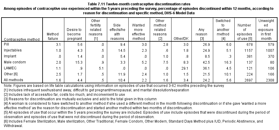
It should be noted that for male condom and LAM/EC the unweighted number of cases (80 and 106 respectively) are too small to present in a report based on the DHS rules for minimum sample sizes. The Other category also has too few cases (166) and at a minimum would be shown in parentheses. We would recommend combining male condom, LAM/EC, and Other into a single "Other methods" category.
Notes and Considerations
Use of contraception is generally not allowed to be missing in any month in the calendar. In the few surveys where it is missing, these are treated as months of non-use of contraception. Missing and unknown reasons for discontinuation are treated as "Other" reasons.
It is worth noting that different assumptions can be made to the calculation of the at risk component of the life table for contraceptive discontinuation. These assumptions are related to the fact that contraceptive information is usually collected using a calendar that collects information on use in calendar months, whereas the life table refers to actual months of use. One consequence of this approach is that censored observations actually contribute a full month of exposure in the last month of observation included in the analysis rather than half a month of exposure. In many life table analyses the number at risk is often taken as the number continuing to the month minus half of the censored observations. For the calculation of discontinuation rates The DHS Program assumes that all observations are at risk for the full month, rather than excluding half the censored observations. Consult Changes over Time in Module 1 for more information on how the calendar has changed over the many phases of The DHS Program.
See also FA59: Model Further Analysis Plan: Contraceptive Use Dynamics (Curtis and Hammerslough, 1995), to provide further ideas and guidance in approaches to manipulating the DHS calendar data.
Next section: Programs and coding resources
Programs
Examples
Programs for all of the examples found in this tutorial are available for Stata and for SPSS, and can be found in the Stata.zip and SPSS.zip files accompanying this tutorial. For Example 1, simple programs are available for R, SAS, CSPro and Excel in addition to the Stata and SPSS examples. Output files for each example are also included in the zip files.
Complete sets of example programs, output and model data can be found at the following links:
| Software | Commands | Input data |
|---|---|---|
| All examples | ||
| Stata | Stata.zip | zzir62fl.dta |
| SPSS | SPSS.zip | zzir62fl.sav |
| Example 1 | ||
| SAS | SAS.zip | zzir62fl.sd2 |
| R | R.zip | zzir62fl.dta |
| CSPro | CSPro.zip | zzir62.dat |
| Excel | Excel.zip | |
Next section: Survey-specific coding
Programs
Survey-specific coding
While the DHS Individual recode datasets follow a standard structure, there is always some survey-specific variation in the coding used. This survey-specific coding can affect the DHS contraceptive calendar data. This section discusses some of the broader survey-specific coding and describes three sets of syntax:
- 1. Realignment of string variables - corrections for calendar and other strings that are left-aligned in some Stata datasets.
- 2. Data fixes - corrections for known problems in datasets.
- 3. Calendar recoding - recoding of method codes and reasons for discontinuation to produce a consistent set of numeric codes across all surveys.
Realignment of string variables
In a small number of Stata datasets, all alphanumeric strings in the dataset were left-aligned at the time the file was constructed. This misalignment affects not only the calendar variables, but also the ID variables such as caseid. The misalignment will cause much of the logic in this tutorial to inaccurately process the calendar data. For most surveys that were affected the datasets were modified and the current Stata datasets are correct16. To check for misalignment of the calendar data, the following code will create a simple tabulation of the first position of the calendar.
gen x=substr(vcal_1,1,1)
tab x
* should be all blank
In all surveys, except one17, this should be blank for all cases, as below. If any other codes show for the variable x, there is a problem of misalignment of the calendar:
          x |      Freq.     Percent        Cum.
------------+-----------------------------------
            |      8,348      100.00      100.00
------------+-----------------------------------
      Total |      8,348      100.00
To check all datasets, use Stata\Calendars shifted.do to process all datasets to look for calendars misaligned.
To correct for any misalignment of data, the do file Stata\Realign vars.do can be used to make the modifications. This do file is set to loop through all of the files known to be misaligned and to correct the alignment of both caseid and the calendar variables vcal_*. Users may prefer to re-download the affected datasets to ensure that the datasets are not misaligned. Corrected versions of the datasets are dated October 29, 2015. The list of datasets that were corrected in 2015 can be found in the do file.
Recommendation: It is recommended that any corrections needed are made to the datasets prior to using them for any analysis.
Data fixes
This section discusses survey-specific modifications to the data needed to successfully process the calendar data. There are two main types of modifications needed:
- 1) Modifications for extended ASCII characters in the calendar.
- 2) Modifications to correct for problems in specific datasets.
Extended ASCII characters:
One of the complications for recoding the survey-specific codes is the alpha codes that have been used in particular surveys. The alpha method and reason codes are generally the letters "A"-"Z" and the numbers "1"-"9" (and "0" meaning not using a method), however in a small number of surveys extended ASCII characters (with ASCII codes 128-255) have been used, principally the codes for "α", "ß", and "Γ" (often displayed as "à", "á", "â"). These codes, though, create a complication in processing in both Stata and SPSS. In most cases the individual recode datasets are saved in pre-Unicode versions of Stata and SPSS, and this means that the codes do not necessarily display well in these software.
For Stata, the Calendar recoding.do file (see below) handles the recoding of these characters, both in versions prior to Unicode (13 and below), and in the Unicode versions (14 and higher).
For SPSS, this is more complicated, and modifications are needed to the data prior to the processing discussed in this tutorial. The SPSS syntax file, Data fixes.sps, contains logic for replacing the internal codes for "α", "ß", and "Γ" (binary pairs of codes with decimal codes 160-162, preceded by decimal code 195) with the characters "$", "%", "&", respectively. The Calendar recoding syntax (see below) then looks for the new codes "$", "%", "&" in the later recoding steps.
Survey-specific issues:
There are a few problems in specific datasets, including the following:
- Dominican Republic DHS 2013 (DRIR21FL) – contains two duplicated cases that are removed prior to further processing.
- Egypt DHS 2005 (EGIR51FL) –
vcal_1contains a code ("Z") in column 1 for a change in source of contraception (not a change in method), and these need to be removed and replaced with the code for the adjacent month for most analyses. - Honduras DHS 2005-06 (HNIR51FL) –
vcal_1contains two cases of code "M" that should be code "B". - Peru DHS 2009 (PEIR5IFL) –
vcal_1contains the incorrect codes for several methods. Codes "F", "L", "8", "9", "E", "M", "*" need to be changed to "C", "F", "L", "8", "9", "E", "M", respectively. - Peru DHS 2012 (PEIR6IFL) – the supplementary variables
v017,v018, andv019are off by 12 months, and are corrected by adding 12 tov017andv018, and subtracting 12 fromv019. Additionally the calendar contains "*" for several months following the month of interview, and needs to be replaced with " ".
Each of these problems is resolved with the logic found in the Data fixes.do file or Data fixes.sps syntax file.
Recommendation: These modifications should be applied immediately after the dataset has been opened and before any other processing of the calendar data. Alternatively, these modifications may be made one time for each relevant dataset and the datasets saved with the modifications in place.
Calendar recoding
In each survey, survey-specific contraceptive method codes or codes for reasons for discontinuation may have been added to the questionnaires. There are no standard codes for these survey-specific methods, and the codes used will vary from survey to survey. For example, several surveys in Indonesia have used added categories for the use of herbs and massage as folkloric contraceptive methods. Additionally, prior to their inclusion as standard methods, some surveys include Emergency Contraception and Standard Days Method as methods of contraception, but used non-standard codes for them. Similarly, surveys have added survey-specific codes for reasons for discontinuation, such as IUD Expelled, Medical Advice, Ramadan, Husband absent/away, in addition to the standard list of reasons.
To facilitate the identification and recoding of these survey-specific codes into a standard set, a Stata do file (Calendar recoding.do) and an SPSS syntax file (Calendar recoding.sps) have been created to help with the recoding.
This calendar recoding will not work when the data are in the original string format (e.g. vcal_1). They are designed to work when the data have been restructured into single months or events, or single months have been extracted through string parsing. This code should be run after the data have been either restructured or extracted. See step 2.7 in Example 2
The calendar recoding routines do three things:
- 1) Set up string variables
methodlistandreasonlistthat contain the list of alpha codes that are used in the calendar for the particular survey, including the survey-specific codes. The character position in this string will represent the numeric code that will later be assigned for that alpha code. For example if themethodlistcontains"123456789WNALCF~M~", the letter "M" is in position 17, indicating that an "M" will later be recoded into code 17 in the resulting numeric variable. The actual list of codes inmethodlistandreasonlistwill be 99 characters in length, mostly filled with tildes (~) as place holders, but permitting the recoding of alpha codes into numeric values from 1 to 99. No actual recoding of data is done in this step – only the creation of survey-specific lists of codes for the methods and reasons. - 2) Recode individual codes for the method (or birth, termination or pregnancy) from a single alpha code into a single numeric code and label the resulting variable with the expanded set of harmonized codes. This step uses the
methodlistcreated in the prior step to determine the numeric codes to assign for the contraceptive method, or the birth, termination or pregnancy. - 3) Recode individual codes for the reason for discontinuation from a single alpha code into a single numeric code and label the resulting variable. This step uses the
reasonlistcreated in the first step to determine the numeric codes to assign for the reason for discontinuation.
The end result of this recoding is that each contraceptive method and each reason for discontinuation has the same numeric value and appropriate label in each dataset.
These calendar recoding routines can be run either without parameters18 (point 1 only) to just produce the lists of survey-specific codes, with parameters for the variable containing the alpha code for the method and a resulting variable for the numeric code (points 1 and 2) to recode just the contraceptive method (and/or pregnancy) codes, or with two additional variables for the alpha code for the reason for discontinuation and a resulting variable for the numeric code (points 1, 2, and 3) to recode both the contraceptive method and the reason for discontinuation codes.
For example, the logic below uses a variable called method_str as the code extracted from a single month from vcal_1, and creates a numeric variable called method_num with the recoded value. The example also uses a variable called reason_str as the code extracted from a single month from vcal_2 for the reason for discontinuation, and creates a numeric variable called reason_num with the recoded numeric value. The calendar recoding routines are used as follows:
run "Calendar recoding.do" method_str method_num reason_str reason_num
* Load the macro for the recoding.
insert file="Calendar recoding.sps".
* recode the method and/or reason for discontinuation.
!Calendar_recoding method_str method_num reason_str reason_num.
Step 2.7 of Example 2 provides sample code (in the comments) to replace the recoding used with the model dataset.
The calendar recoding also recodes the births, terminated pregnancies, and other months of pregnancy into numeric codes 81, 82, and 83, respectively, as well as recoding the contraceptive methods.
Recommendation: The Calendar recoding.do or Calendar recoding.sps should be run from within the example code when a single month method code or reason for discontinuation code is to be recoded to a numeric code. This recoding cannot be used to recode all months of the calendar at the same time – it only works for a single month at a time.
16. Note, though, that the version number of the dataset was not updated and users that had previously downloaded the dataset may not be aware of the modified version. For almost all of the corrected datasets the date of the modified dataset is 10/29/2015.
17. In the Maldives 2009 DHS (MVIR52FL.dta) there are 7 cases with non-blank codes in the first position.
18. Parameters here are variables passed to the Calendar recoding routines for 1) the alpha method code variable, 2) the resulting numeric method variable, 3) the alpha reason for discontinuation code variable, and 4) the resulting numeric reason for discontinuation variable.
Next section: Acknowledgments
Annexes
Acknowlegements
The DHS Contraceptive Calendar Tutorial was prepared by Trevor Croft with key inputs from Sarah Bradley and Courtney Allen. The initial outline was prepared by Sarah Bradley and Trevor Croft, with substantive ideas from Sarah Staveteig and Kerry MacQuarrie. The design of the tutorial was based on suggestions from a number of DHS Contraceptive Calendar users including Yoonjoung Choi, Sarah Staveteig, and Kerry McQuarrie, as well as several questions and comments received through the DHS User Forum. The text of the tutorial was drafted by Trevor Croft with some sections written by Sarah Bradley and Courtney Allen. Examples were prepared by Trevor Croft in both Stata and SPSS largely based on program logic previously prepared or on Stata program logic provided by Sarah Bradley, Sarah Staveteig, and Tesfayi Gebreselassie. The examples were tested by Courtney Allen and Aileen Marshall. The tutorial videos were written and narrated by Courtney Allen and produced by Cameron Taylor. The web pages were prepared by Trevor Croft, Bob Bozsa and Aileen Marshall.
The full tutorial and examples were reviewed by Courtney Allen and Aileen Marshall. Sarah Bradley, Younjoung Choi, Ewa Batyra, Peter Kisaakye, Suzanne Bell, Wafaa Soliman, German Rodriguez, Bill Winfrey, and Stan Becker provided written feedback and comments on the tutorial and examples.
A special thanks to the staff and students of the Bill & Melinda Gates Institute for Population and Reproductive Health at Johns Hopkins Bloomberg School of Public Health, and to colleagues at the DHS Program who attended seminars covering parts of the tutorial and gave thoughtful ideas on the content and design of the tutorial.
Next section: References
Annexes
References
Model Further Analysis Plan: Contraceptive Use Dynamics. Sian L. Curtis and Charles R. Hammerslough. FA59. 1995. http://dhsprogram.com/publications/publication-FA59-Further-Analysis.cfm
Determinants of Contraceptive Failure, Switching, and Discontinuation: An Analysis of DHS Contraceptive Histories. Sian L. Curtis and Ann K. Blanc. AR6. 1997. http://dhsprogram.com/publications/publication-AR6-Analytical-Studies.cfm
Studies in Family Planning. 2002 June;33(2):127-40. Monitoring contraceptive continuation: links to fertility outcomes and quality of care. Blanc AK, Curtis SL, Croft TN.
Levels, Trends, and Reasons for Contraceptive Discontinuation. Sarah E.K. Bradley, Hilary M. Schwandt, Shane Khan. AS20. 2009. http://dhsprogram.com/publications/publication-AS20-Analytical-Studies.cfm
Contraceptive use and perinatal mortality in the DHS: an assessment of the quality and consistency of calendars and histories. Bradley, Sarah E.K., William Winfrey, and Trevor N. Croft. MR17. 2015. http://www.dhsprogram.com/publications/publication-MR17-Methodological-Reports.cfm
Cleland J, Ali MM, and Shah I. 2006. "Dynamics of contraceptive use", in: UN Department of Economic and Social Affairs, Population Division, Levels and Trends of Contraceptive Use as Assessed in 2002, pp. 87-115, Table 22, page 98. http://www.un.org/esa/population/publications/wcu2002/WCU2002_Report.pdf
MacQuarrie, Kerry L.D., Sarah E.K. Bradley, Alison Gemmill, and Sarah Staveteig. 2014. Contraceptive Dynamics Following HIV Testing. DHS Analytical Studies No. 47. Rockville, Maryland, USA: ICF International. http://dhsprogram.com/publications/publication-AS47-Analytical-Studies.cfm
Staveteig, Sarah, Lindsay Mallick, and Rebecca Winter. 2015. Uptake and Discontinuation of Long-Acting Reversible Contraceptives (LARCs) in Low-Income Countries. DHS Analytical Studies No. 54. Rockville, Maryland, USA: ICF International. http://www.dhsprogram.com/publications/publication-as54-analytical-studies.cfm
MacQuarrie, Kerry L.D., Lindsay Mallick, and Sunita Kishor. 2016. Intimate Partner Violence and Interruption to Contraceptive Use. DHS Analytical Studies No. 57. Rockville, Maryland, USA: ICF International. http://www.dhsprogram.com/publications/publication-as57-analytical-studies.cfm
History of the calendar:
Dominican Republic: 1986 - Dominican Republic 1986 Final Report (Experimental). http://dhsprogram.com/publications/publication-FR11-Other-Final-Reports.cfm
Peru: 1986 - Peru 1986 Final Report (Experimental). http://dhsprogram.com/publications/publication-FR32-Other-Final-Reports.cfm
Collection of survey data on contraception: an evaluation of an experiment in Peru. Goldman N, Moreno L, Westoff CF. Studies in Family Planning. 1989 May-June;20(3):147-57.
Use of a monthly calendar for collecting retrospective data on contraception: an evaluation of the experimental field studies of the Demographic and Health Surveys (DHS). [Article in Spanish] Moreno L, Goldman N, Babakol O. Notas Poblacion. 1991 Apr;18-19(51-52):11-37.